Time-Lapse Imaging as an Inverse Problem

Claerbout (2004); Tarantola (1987) discuss the use of geophysical inversion as an imaging tool. In recent applications, inverted seismic images are computed by weighting the migration result with the inverse of the Hessian matrix. The associated large computational cost and complexity makes the explicit computation of the Hessian matrix and its inverse impracticable. Valenciano et al. (2006) demonstrate that by taking the sparsity of the Hessian into account, the inverse of the Hessian matrix may be computed cheaply and applied in a target-oriented manner. This approach appears to yield better results than simple migration in subsalt reservoirs. For the time-lapse problem, one approach would be to to compute the time-lapse image as a difference between inverse images computed as described above. Another approach would be to solve for the time-lapse image through inversion rather a difference between images.

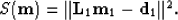
Given a linear modeling operator ${\bf L}$, the synthetic data d is computed using ${\bf d}={\bf L}{\bf m}$, where m is a reflectivity model. Two different surveys (say a baseline and monitor) may be represented as follows:  

$${\bf L}{\bf m}_{0}={\bf d}_{0}, \nonumber$$

$${\bf L}{\bf m}_{1}={\bf d}_{1},$$ (1)

where ${\bf m}_{0}$ and ${\bf m}_{1}$ are the reflectivity models at the time we acquire the datasets, (${\bf d}_{0}$ and ${\bf d}_{1}$) respectively. Taking ${\bf L}_{0}$ and ${\bf L}_{1}$ to be the modeling operators for two different surveys, the quadratic cost functions are defined as  

$$S({\bf m})=\Vert {\bf L}_{0}{\bf m}_{0} - {\bf d}_{0} \Vert^2, \nonumber$$

 

$$S({\bf m})=\Vert {\bf L}_{1}{\bf m}_{1} - {\bf d}_{1} \Vert^2.$$ (2)

The least-squares solutions to the problems are given as

$$\hat{{\bf m}}_{0}=({\bf L}'_{0}{\bf L}_{0})^{-1}{\bf L}'_{0}... ...de {\bf m}_{0}= {\bf H}_{0}^{-1} \tilde {\bf m}_{0}, \nonumber$$

$$\hat{{\bf m}}_{1}=({\bf L}'_{1}{\bf L}_{1})^{-1}{\bf L}'_{1}... ...)^{-1} \tilde {\bf m}_{1}= {\bf H}_{1}^{-1} \tilde {\bf m}_{1},$$ (3)

where $\tilde {\bf m}_{0}$ and $\tilde {\bf m}_{1}$ are the migrated images, $\hat{{\bf m}}_{0}$ and $\hat{{\bf m}}_{1}$ are the least-squares inverse images, ${\bf L}'_{0}$ and ${\bf L}'_{1}$ are the migration operators, while ${\bf H}_{0}={\bf L}'_{0}{\bf L}_{0}$ and ${\bf H}_{1}={\bf L}'_{1}{\bf L}_{1}$ are the Hessian matrices.

In the first approach, the inverse time-lapse image ($\Delta \hat{{\bf m}}$) is given by

$$\Delta \hat{{\bf m}}= \hat{{\bf m}}_{1} - \hat{{\bf m}}_{0}.$$ (4)

In the second approach, we express the modeling of operation for the two surveys as follows:

$${\bf L}_{0}{\bf m}_{0} = {\bf d}_{0}, \nonumber$$

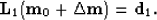$${\bf L}_{1}({\bf m}_{0} + \Delta {\bf m} ) = {\bf d}_{1}.$$ (5)

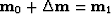where ${\bf m}_{0} + \Delta {\bf m} = {\bf m}_{1}$. In matrix form, we can write  

$$\left [ \begin{array} {cc} {\bf L}_{0} & 0 \\ {\bf L}_{1} &... ...n{array} {cc} {\bf d}_{0} \\ {\bf d}_{1} \end{array} \right ].$$ (6)

least-squares solution to equation 10 is given as  

$$\left [ \begin{array} {cc} {\bf L}'_{0} {\bf L}_{0}+{\bf L}'... ...\tilde {\bf m}_{1} \\ \tilde {\bf m}_{1} \end{array} \right ],$$ (7)

 

$$\left [ \begin{array} {cc} {\bf H}_{0}+{\bf H}_{1} & {\bf H}... ...\tilde {\bf m}_{1} \\ \tilde {\bf m}_{1} \end{array} \right ].$$ (8)

This, may be re-arranged as follows:  

$$\left [ \begin{array} {cc} \hat{{\bf m}}_{0} \\ \Delta \hat... ...\tilde {\bf m}_{1} \\ \tilde {\bf m}_{1} \end{array} \right ].$$ (9)