Interpolation with non-stationary PEFs

Interpolation can be cast as a series of two inverse problems where a prediction-error filter is estimated on known data and is then used to interpolate missing data. A prediction-error filter (PEF) can be estimated by minimizing the output of convolution of known data with an unknown filter (except for the leading 1), which can be written in matrix form as  

$$\bold 0 \quad \approx \quad \bold r = \left[ \begin{array} {... ... {c} d_2 \\ d_3 \\ d_4 \\ d_5 \\ d_6 \end{array} \right] ,$$ (2)

where f_i are unknown filter values and d_i are known data values.

The filters used in this paper are all multidimensional, which are computed with the helical coordinate. In the case of a stationary multidimensional PEF, this is an over-determined least-squares problem with a unique solution.

Seismic data is non-stationary in nature, so a single stationary PEF is not adequate for changing dips. I estimate a single spatially-variable non-stationary PEF and solve a global optimization problem Guitton (2003). In that case the problem is under-determined, and a regularization term is added to the least-squares problem so that (in matrix notation),

$$\begin{eqnarray} \bold{DKf} + \bold{d} \approx \bold{0} \nonumber \\ \epsilon \bf A f \approx 0 ,\end{eqnarray}$$ (3)

where $\bf{D}$ represents non-stationary convolution with the data, $\bf{f}$ is now a non-stationary PEF, $\bf{K}$ (a selector matrix) and $\bf{d}$ (a copy of the data) both constrain the value of the first filter coefficient to 1, $\bf{A}$ is a regularization operator (a Laplacian operating over space) and $\epsilon$ is a trade-off parameter for the regularization. Solving this system will create a smoothly variable PEF.

Once the PEF has been estimated, it can be used in a second least squares problem that matches the output model to the known data while simultaneously regularizing the model with the newly found PEF,

$$\begin{eqnarray} \bold{S(m - d)} = \bold{0} \nonumber\\ \bf F m \approx 0 ,\end{eqnarray}$$ (4)

where $\bf{S}$ is a selector matrix which is 1 where data is present and where it is not, $\bf{F}$ represents convolution with the non-stationary PEF, and $\bf{m}$ is the desired model.

 

pseudo2
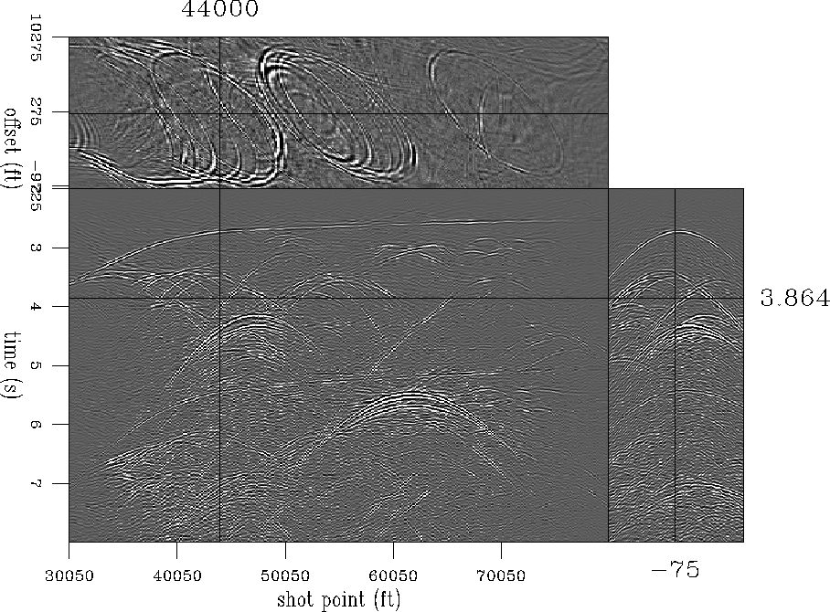
Figure 4 Pseudo-primaries located on a missing common-offset section from the input data set.