

Next: Interpolation with non-stationary PEFs
Up: Curry: Interpolation with pseudo-primaries:
Previous: INTRODUCTION
Pseudo-primaries can be generated by computing a slightly modified version of
cross-correlation of primaries and a multiple model Shan and Guitton (2004)
|  |
(1) |
where W is the pseudo-primary data,  is frequency, xs
is the shot location, xp and xm are receiver locations,
  is the complex
conjugate of the original trace at (xs,xp) and
  is that same
data at xm. In this equation, the result of the cross-correlation of primaries,
first-order multiples and second-order multiples in D are outlined in the table below, with
the first and second columns corresponding to the inputs to the cross-correlation
and the third column corresponding to the output.
| Input 1 |
Input 2 |
Output |
| first-order multiples |
first-order multiples |
zero-lag |
| second-order multiples |
second-order multples |
zero-lag |
| first-order multiples |
primaries |
pseudo-primaries |
| second-order multiples |
first-order multiples |
pseudo-primaries |
| second-order multiples |
primaries |
pseudo-first-order multiples |
With higher order multiples the trend in this table continues.
This produces similar results to cross-correlating primaries with a
multiple model Shan and Guitton (2004), as the additional correlation
of the primaries on one term is already taking place with the identical
primaries on the other term of the autocorrelation.
Pseudo-primaries generated in this fashion contain subsurface
information that would not be recorded with a non-zero minimum offset.
One example of this is a first-order multiple that reflects at the free
surface within the recording array, resulting in near offsets being
recorded when that wave returns to the surface. This is
shown in Figures ![[*]](http://sepwww.stanford.edu/latex2html/cross_ref_motif.gif) and
and ![[*]](http://sepwww.stanford.edu/latex2html/cross_ref_motif.gif) , where Figure
, where Figure ![[*]](http://sepwww.stanford.edu/latex2html/cross_ref_motif.gif) is a cube of the input Sigsbee2B shots (including the negative offsets
predicted by reciprocity) but with offsets less than 2000 feet
removed, and Figure
is a cube of the input Sigsbee2B shots (including the negative offsets
predicted by reciprocity) but with offsets less than 2000 feet
removed, and Figure ![[*]](http://sepwww.stanford.edu/latex2html/cross_ref_motif.gif) is the corresponding cube of pseudo-primaries for the same
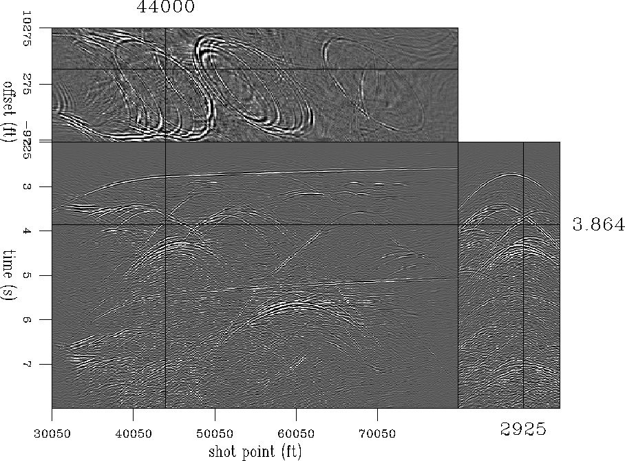
area. Put briefly, the source coverage of the pseudo-primary data is much greater than that
of the input data because all receivers in the original data become sources
for the pseudo-primaries.
is the corresponding cube of pseudo-primaries for the same
area. Put briefly, the source coverage of the pseudo-primary data is much greater than that
of the input data because all receivers in the original data become sources
for the pseudo-primaries.
input
Figure 1 Input dataset missing the nearest 2000' of offsets on either side.


 pseudo
Figure 2 Pseudo-primaries created by autocorrelation and summation of Figure
![[*]](http://sepwww.stanford.edu/latex2html/cross_ref_motif.gif) . Note that the near offsets have been filled in.
. Note that the near offsets have been filled in.


Figure ![[*]](http://sepwww.stanford.edu/latex2html/cross_ref_motif.gif) contains a lot of near-offset information present in the
pseudo-primaries that is not present in the recorded primaries.
However, simply replacing the missing near offsets of the primaries with
the corresponding pseudo-primaries would not yield a satisfactory result
due to the crosstalk and noise in the pseudo-primaries.
contains a lot of near-offset information present in the
pseudo-primaries that is not present in the recorded primaries.
However, simply replacing the missing near offsets of the primaries with
the corresponding pseudo-primaries would not yield a satisfactory result
due to the crosstalk and noise in the pseudo-primaries.
pseudoex
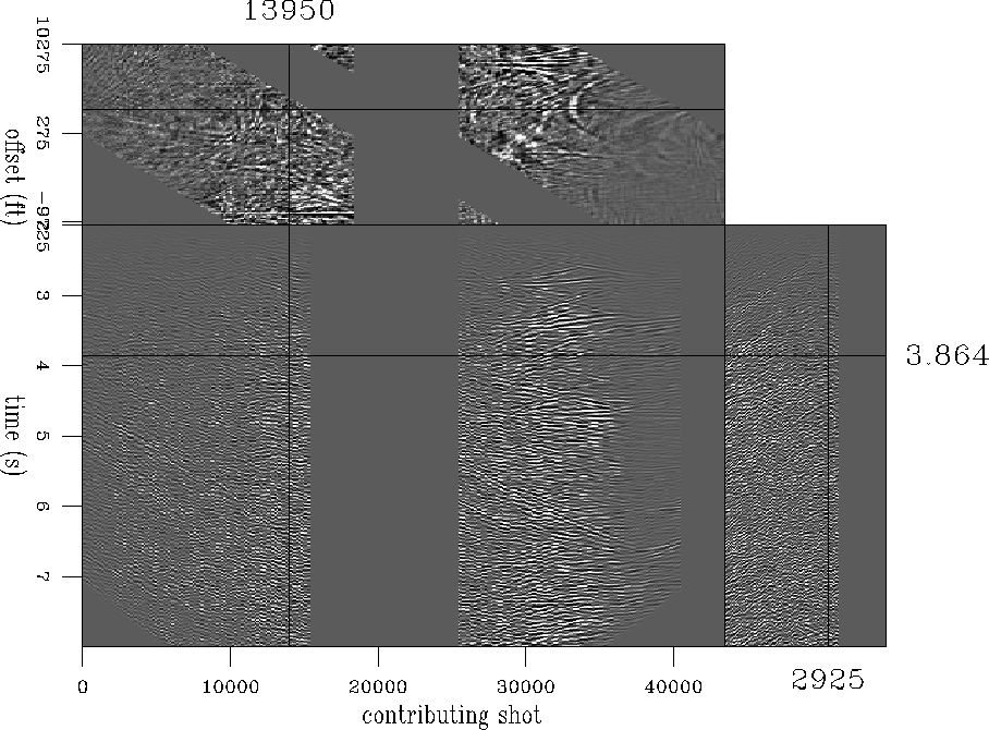
Figure 3 A single virtual shot from figure ![[*]](http://sepwww.stanford.edu/latex2html/cross_ref_motif.gif) that has been expanded over the input shot axis.
that has been expanded over the input shot axis.


The crosstalk in the pseudoprimaries is largely a function of the number of shots that are summed
over in the input data. Figure ![[*]](http://sepwww.stanford.edu/latex2html/cross_ref_motif.gif) shows the shot on the right panel of Figure
shows the shot on the right panel of Figure ![[*]](http://sepwww.stanford.edu/latex2html/cross_ref_motif.gif) , but
without the summing over shots in equation 1 where instead of summing over shots
each shot is plotted along the front face of the cube. It shows how the stacking procedure greatly increases the signal-to-noise ratio.
, but
without the summing over shots in equation 1 where instead of summing over shots
each shot is plotted along the front face of the cube. It shows how the stacking procedure greatly increases the signal-to-noise ratio.


Next: Interpolation with non-stationary PEFs
Up: Curry: Interpolation with pseudo-primaries:
Previous: INTRODUCTION
Stanford Exploration Project
5/6/2007
![[*]](http://sepwww.stanford.edu/latex2html/cross_ref_motif.gif) and
and ![[*]](http://sepwww.stanford.edu/latex2html/cross_ref_motif.gif) , where Figure
, where Figure ![[*]](http://sepwww.stanford.edu/latex2html/cross_ref_motif.gif) is a cube of the input Sigsbee2B shots (including the negative offsets
predicted by reciprocity) but with offsets less than 2000 feet
removed, and Figure
is a cube of the input Sigsbee2B shots (including the negative offsets
predicted by reciprocity) but with offsets less than 2000 feet
removed, and Figure ![[*]](http://sepwww.stanford.edu/latex2html/cross_ref_motif.gif) is the corresponding cube of pseudo-primaries for the same
area. Put briefly, the source coverage of the pseudo-primary data is much greater than that
of the input data because all receivers in the original data become sources
for the pseudo-primaries.
is the corresponding cube of pseudo-primaries for the same
area. Put briefly, the source coverage of the pseudo-primary data is much greater than that
of the input data because all receivers in the original data become sources
for the pseudo-primaries.


![[*]](http://sepwww.stanford.edu/latex2html/cross_ref_motif.gif) . Note that the near offsets have been filled in.
. Note that the near offsets have been filled in.
![[*]](http://sepwww.stanford.edu/latex2html/cross_ref_motif.gif) contains a lot of near-offset information present in the
pseudo-primaries that is not present in the recorded primaries.
However, simply replacing the missing near offsets of the primaries with
the corresponding pseudo-primaries would not yield a satisfactory result
due to the crosstalk and noise in the pseudo-primaries.
contains a lot of near-offset information present in the
pseudo-primaries that is not present in the recorded primaries.
However, simply replacing the missing near offsets of the primaries with
the corresponding pseudo-primaries would not yield a satisfactory result
due to the crosstalk and noise in the pseudo-primaries.

![[*]](http://sepwww.stanford.edu/latex2html/cross_ref_motif.gif) that has been expanded over the input shot axis.
that has been expanded over the input shot axis.
![[*]](http://sepwww.stanford.edu/latex2html/cross_ref_motif.gif) shows the shot on the right panel of Figure
shows the shot on the right panel of Figure ![[*]](http://sepwww.stanford.edu/latex2html/cross_ref_motif.gif) , but
without the summing over shots in equation 1 where instead of summing over shots
each shot is plotted along the front face of the cube. It shows how the stacking procedure greatly increases the signal-to-noise ratio.
, but
without the summing over shots in equation 1 where instead of summing over shots
each shot is plotted along the front face of the cube. It shows how the stacking procedure greatly increases the signal-to-noise ratio.