|
VelSpec-slice-rho.99-taylor-taylor-flat
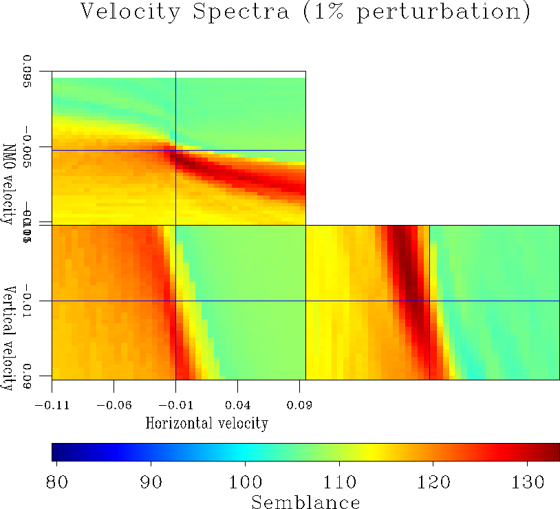
Figure 6 Velocity Spectra obtained when a constant anisotropic velocity was perturbed by |  |
|
VelSpec-slice-rho.99-taylor-taylor-flat
Figure 6 Velocity Spectra obtained when a constant anisotropic velocity was perturbed by |  |
|
VelSpec-slice-rho.9-taylor-taylor-flat
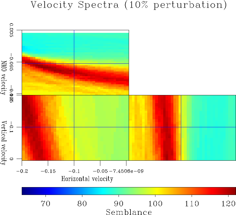
Figure 7 Velocity Spectra obtained when a constant anisotropic velocity was perturbed by |  |
Figures 6 and 7 illustrate that the anisotropic velocity spectra provide accurate estimates of the velocity parameters for small initial velocity perturbations. The accuracy of the estimates then deteriorates as the initial velocity perturbation increases. The bias in the perturbation estimates is due to the fact that the linearized expression of the residual moveout is only a first-order approximation. As illustrated in figures 4 and 5, the linearized formula underestimates the real moveout. Consequently, perturbation estimates from the velocity spectra are of larger magnitude than the true initial perturbations.
Furthermore, the different slices of the velocity spectra show that vertical velocity is by far
the most poorly constrained parameter. However, assuming the vertical velocity is
determined, the upper panel shows a trade-off between the estimates of ![]() and
and ![]() that is
approximately linear.
that is
approximately linear.
Finally, we estimate the initial anisotropic migration velocity perturbations,
=![]() ,by picking the maxima of the semblance cubes, =
,by picking the maxima of the semblance cubes, =![]() . The
updated velocity parameters are given by
. The
updated velocity parameters are given by ![]() ,where
,where ![]() is the vector of starting
anisotropic migration velocities. It is then possible to remigrate the data with our new
estimates of the anisotropic parameters and proceed to a new MVA. Note that after MVA, the
the new perturbation,
is the vector of starting
anisotropic migration velocities. It is then possible to remigrate the data with our new
estimates of the anisotropic parameters and proceed to a new MVA. Note that after MVA, the
the new perturbation, ![]() is given by
is given by ![]() .
.
The following table illustrates the results of the updating process for the two different synthetic cases presented above. It shows that the overall estimation of the anisotropic parameters after picking the maxima of the semblance cubes.
| Perturbation | Starting | Picked | Updated |
|---|---|---|---|
| perturbation | perturbation | perturbation | |
| 1% Perturbation | |||
| 10% Perturbation |