[3] The meaning and calculation of $\nabla f\left( \delta m \right)$ and $\nabla^{2} f\left( \delta m \right)$

The iterative formula of the least-squares migration/inversion is:  

$$\delta \textbf{m}^{\left( k+1\right) }=\delta \textbf{m}^{\l... ...\right) } -H^{k+1}\nabla f\left(\delta \textbf{m}^{(k)}\right),$$ (74)

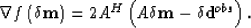
where H^k+1 is the inverse of the Hessian. The first-order derivative $\nabla f\left(\delta \textbf{m}^{(k)}\right)$ of the cost function with respect to the medium parameters is  

$$\nabla f\left(\delta \textbf{m} \right) =2 A^{H}\left(A\delta \textbf{m} - \delta \textbf{d}^{obs} \right).$$ (75)

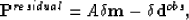
If the residual wavefield is defined as  

$$\textbf{P}^{residual} = A\delta \textbf{m} - \delta \textbf{d}^{obs},$$ (76)

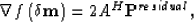
and equation (75) is rewritten as  

$$\nabla f\left(\delta \textbf{m} \right) =2 A^{H}\textbf{P}^{residual},$$ (77)

then the first-order derivative means that the residual wavefield is back-propagated. It is further equivalent to the classical prestack migration if the parameter disturbance $\delta \textbf{m}$ is set to zero at the first iteration. The residual wavefield $\textbf{P}^{residual}$ belongs to the data space $D\left(\vec{x}_{r}, \vec{x}_{s}, t \right)$, and $\nabla f\left(\delta \textbf{m} \right)$ pertains to the image space $I\left(\vec{x} \right)$.Calculating the first-order derivative requires one-time modeling $A\delta \textbf{m}$, which can be implemented by a prestack demigration, and one-time classical prestack migration of $2 A^{H}\textbf{P}^{residual}$:

$$\begin{eqnarray} \nabla f\left(\delta \textbf{m} \right) =&2&\left[ \begin{array... ...e{g}^{D}_{2N} & \cdots & \tilde{g}^{D}_{QN} \\ \end{array}\right].\end{eqnarray}$$ (78)

In the first iterative step, $\delta \textbf{m}=0$, equation (78) is rewritten as

$$\begin{eqnarray} \nabla f\left(\delta \textbf{m} \right) &=&-2\left[ \begin{arra... ...otfill \\ r_{P1} & r_{P2} & \cdots & r_{PQ} \\ \end{array}\right].\end{eqnarray}$$ (79)

The Hessian is the second-order derivative of the cost function with respect to the medium parameters. It is of the following form:  

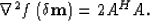$$\nabla^{2} f\left(\delta \textbf{m} \right) =2 A^{H}A .$$ (80)

In the least-squares migration/inversion, the Hessian is a deconvolution operator. It is used for de-blurring the image of the classical prestack migration. Physically, the Hessian is an indicator of the illumination. The energy of the wave propagating through a certain medium is expressed as follows:  

$$E\left(\delta \textbf{m} \right)=\Vert \delta \textbf{d}\Ver... ...U} \right] \left[\delta \textbf{m} \right]\left[W^{D} \right] .$$ (81)

For a given layer and from the modeling equation (58), equation (81) can be rewritten as

$$\begin{eqnarray} E\left(\delta \textbf{m} \right) &=&\left[\begin{array} {llcl} ... ...D}_{Q1} & g^{D}_{Q2} & \cdots & g^{D}_{QN} \\ \end{array}\right]. \end{eqnarray}$$ (82)

Clearly, for a horizontal reflector with an even reflectivity and only the zero-offset reflectivity considered, A^HA determines the energy of the wave which propagates to the layer. Equation (82) can be rewritten as follows:

$$\begin{eqnarray} A^{H}A&=&\left[W^{D} \right] ^{H} \left[W^{U} \right]^{H} \left... ...}_{Q1} & g^{D}_{Q2} & \cdots & g^{D}_{QN} \\ \end{array}\right] . \end{eqnarray}$$ (83)

The row in the matrix $\left[ W^{U} \right]^{H}$ multiplied by the column of the matrix $\left[ W^{U}\right]$ and the row in the matrix $\left[W^{D} \right]$ multiplied by the column of the matrix $\left[ W^{D} \right]^{H}$ are the cross-correlation between the conjugate of the Green's function and the Green's function at different receiver or shot positions respectively. The auto-correlation has a peak value, and the cross-correlation decreases rapidly as the distance increases between the receiver and shot positions. The auto-correlation values are on the diagonal. Therefore, the Hessian is a band-width-limited diagonal matrix. Its inverse is also a kind of band-width-limited diagonal matrix. In the extreme case, where only the elements on the diagonal of the Hessian are left, with non-diagonal set to zero, the elements on the diagonal of the inverse of the Hessian are the reciprocals of the elements on the diagonal of the Hessian. Therefore, the inverse of the Hessian plays the role of decreasing strong illumination and enhancing poor illumination. The Hessian itself reflects the illumination of each imaging point. The matrix expression of migration/inversion can be summarized as follows:

$$\begin{eqnarray} &&\left[ \begin{array} {llcl} r_{11} & r_{12} & \cdots & r_{1Q}... ... g^{D}_{QN} \\ \end{array}\right]\right\rbrace ^{-1} _{Q\times Q}.\end{eqnarray}$$ (84)

Substituting the residual imaging matrix into equation (84), it can be rewritten as follows:

$$\begin{eqnarray} &&\left[ \begin{array} {llcl} r_{11} & r_{12} & \cdots & r_{1Q}... ... g^{D}_{QN} \\ \end{array}\right]\right\rbrace ^{-1} _{Q\times Q}.\end{eqnarray}$$ (85)

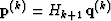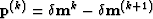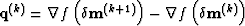With the quasi-Newton condition $\textbf{p}^{(k)}=H_{k+1}\textbf{q}^{(k)}$, and $\textbf{p}^{(k)}=\delta \textbf{m}^{k}-\delta \textbf{m}^{(k+1)}$, $\textbf{q}^{(k)}=\nabla f\left(\delta \textbf{m}^{(k+1)}\right) - \nabla f\left(\delta \textbf{m}^{(k)}\right)$, the DFP algorithm for calculating the inverse of the Hessian matrix is  

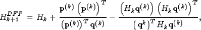$$H^{DFP}_{k+1}=H_{k}+\frac{ \textbf{p}^{(k)}\left(\textbf{p}^... ...)^{T}}{\left(\textbf{q}^{k} \right)^{T}H_{k}\textbf{q}^{(k)}} ,$$ (86)

where  

$$\textbf{p}^{(k)}=\left[ \begin{array} {llcl} r_{11} & r_{12}... ...\\ r_{P1}& r_{P2} & \cdots & r_{PQ} \\ \end{array}\right]^{k+1}$$ (87)

and

$$\begin{eqnarray} \textbf{q}^{(k)}&=&\left[ 2 A^{H}\textbf{P}^{residual} \right] ... ...{residual} & \cdots & r_{PQ}^{residual} \\ \end{array}\right]^{k},\end{eqnarray}$$ (88)

where r_ij^residual is the image with the residual wavefield.
 

• [4] Analysis of some factors that influence imaging
• [5] The imaging gather of migration/inversion
• [6] The resolution of migration/inversion
• [7] The regularization of the migration/inversion algorithms
• [8] The convergence of the iterative migration/inversion