Adaptive filtering with non-stationary helical filters

To handle the inherent non-stationarity of seismic data, I estimate a bank of non-stationary filters using helical boundary conditions Claerbout (1998); Mersereau and Dudgeon (1974). This approach has been successfully utilized by Rickett et al. (2001) to attenuate surface-related multiples. As described before [equation ()], I use the Huber norm to approximate the $\ell^1$ norm and a standard conjugate-gradient solver with the $\ell^2$ norm. The filter coefficients vary smoothly across the output space by introducing a regularization term inside equation () Crawley (2000); Rickett et al. (2001). The misfit function to minimize becomes  

$$e_1({\bf f})=\vert{\bf Mf}-{\bf d}\vert _{Huber}+\epsilon^2\Vert{\bf Rf}\Vert^2,$$ (13)

 

interl2
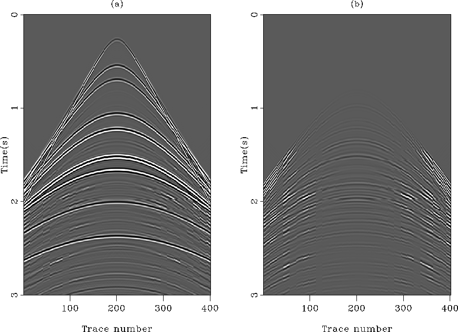
Figure 7 (a) The estimated primaries with the $\ell^2$ norm. (b) The estimated internal multiples with the $\ell^2$ norm. Ideally, (b) should look like Figure b, but it does not.

 

interl1
Figure 8 (a) The estimated primaries with the $\ell^1$ norm. (b) The estimated internal multiples with the $\ell^1$ norm. Beside some edge-effects, (b) resembles closely Figure b. The adaptive subtraction worked very well.

where ${\bf f}$ is the unknown vector of filter coefficients for the non-stationary matching filters and ${\bf R}$ is a regularization operator. The Helix derivative Claerbout (1998) is chosen for ${\bf R}$.In the following results, the non-stationary filters are 1-D. The same number of coefficients per filter are estimated with both $\ell^2$ and $\ell^1$ norms.