


![[*]](http://sepwww.stanford.edu/latex2html/cross_ref_motif.gif) a shows the estimated primaries when the b displays
the estimated internal multiples.
As expected, because of the local amplitude
differences between the signal (primaries) and the noise (multiples), the
adaptive subtraction fails and we retrieve the behavior explained in the preceding
section with the 1-D example. Now, in Figure , we see the
beneficial effects of the a shows
the estimated primaries and Figure b the estimated
multiples. The noise subtracted matches very well the
internal multiple model in Figure b, as anticipated.
Note that with this dataset,
a shows the estimated primaries when the b displays
the estimated internal multiples.
As expected, because of the local amplitude
differences between the signal (primaries) and the noise (multiples), the
adaptive subtraction fails and we retrieve the behavior explained in the preceding
section with the 1-D example. Now, in Figure , we see the
beneficial effects of the a shows
the estimated primaries and Figure b the estimated
multiples. The noise subtracted matches very well the
internal multiple model in Figure b, as anticipated.
Note that with this dataset, 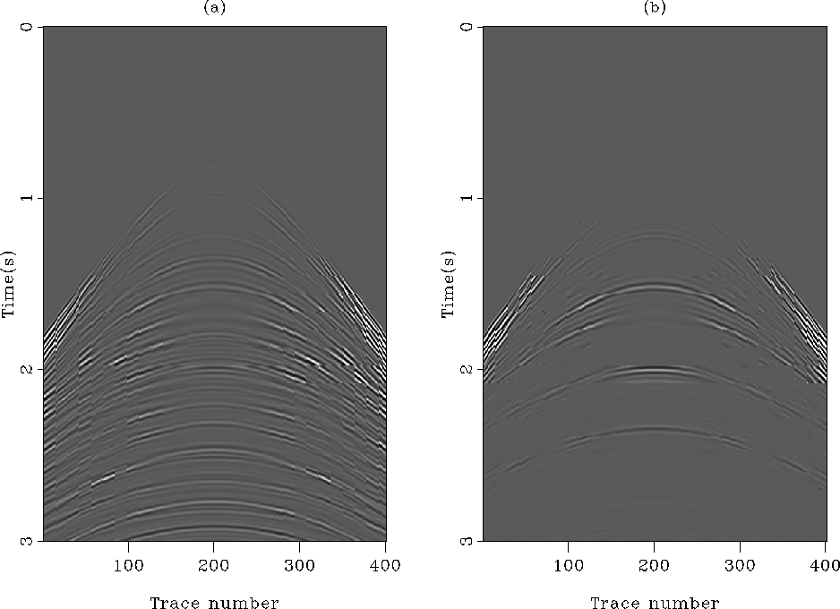 |
b) and the subtracted
multiples with the b) and the subtracted
multiples with the 


As a final comparison, Figure displays the
difference between the internal-multiple model (Figure
b) and the subtracted multiples with the two norms. The
![]() norm (Figure b) matches the multiple
model much better than the
norm (Figure b) matches the multiple
model much better than the ![]() norm (Figure
a).
norm (Figure
a).