Shaping filters and the $\ell^1$ norm

The strong primary in Figure can be seen as an outlier that attracts much of the solver's efforts during the filter estimation.

 

filterl2 Figure 3 Shaping filter estimated for the 1-D problem with the 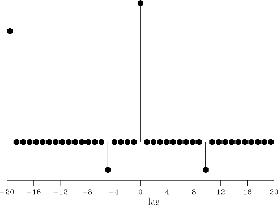$\ell^2$ norm. This filter is not a single spike at lag=0.

 

filterl1 Figure 4 Shaping filter estimated for the 1-D problem with the 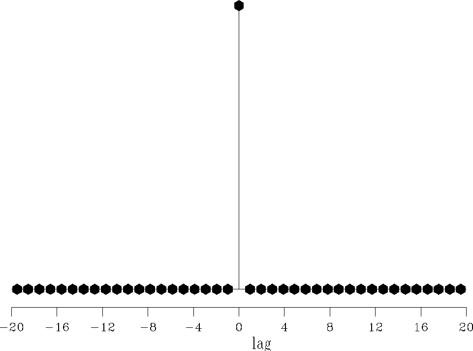$\ell^1$ norm. This filter is a single spike at lag=0.

Consequently, some of the signal leaks into the noise. Because the $\ell^1$ norm is robust to outliers, I propose estimating the filter coefficients with it. This insensitivity to large ``noise'' has a statistical interpretation: robust measures are related to long-tailed density functions in the same way that $\ell^2$is related to the short-tailed gaussian density function Tarantola (1987). In this section, I show that the $\ell^1$ norm solves the problem highlighted in the preceding section.

Now our goal is to estimate one shaping filter ${\bf f}$ that minimizes the objective function  

$$e_1({\bf f})=\vert{\bf Mf}-{\bf d}\vert _{\ell^1} .$$ (10)

The function in equation () is singular where any residual component vanishes implying that the derivative of $e_1({\bf f})$ is not continuous everywhere. Unfortunately, most of our optimization techniques, e.g., conjugate-gradient or Newton methods, assume that the first derivative of the objective function is continuous in order to find its minimum. Therefore, specialized techniques have been developed to either minimize or approximate the $\ell^1$ norm. For instance, various approaches based on a linear programming viewpoint have been used with success, e.g., Barrodale and Roberts 1980. Another idea is to minimize a hybrid $\ell^1/\ell^2$ norm with an iteratively reweighted least-squares (IRLS) method Bube and Langan (1997); Gersztenkorn et al. (1986); Scales and Gersztenkorn (1988).

Alternatively, the Huber norm is utilized. This technique yields a good approximation of the $\ell^1$ norm. Therefore, the objective function we minimize becomes  

$$e_1({\bf f})=\vert{\bf Mf}-{\bf d}\vert _{Huber},$$ (11)

The minimization of the Huber norm is performed with a quasi-Newton method (Appendix ). The only parameter that needs to be set is $\alpha$ in equation (). Consistent with the strategy of Chapter , I set

$$\alpha = \frac{max\vert\bold{d}\vert}{100}.$$ (12)

From now on, I call $\ell^1$ norm the Huber norm. In text section, I show that the $\ell^1$ norm leads to the desired result for the filter estimation problem.