Introduction

Robust error measures such as the $\ell^1$ norm have found a number of applications in geophysics. As measures of data misfit, they show considerably less sensitivity to large measurement errors than least-squares ($\ell^2$) measures. Since geophysical inverse problems are generally ill-posed, relatively noise insensitive misfit measures can yield far more stable estimates of Earth parameters than does $\ell^2$ norm Chapman and Barrodale (1983); Claerbout and Muir (1973); Scales and Gersztenkorn (1987); Scales et al. (1988); Taylor et al. (1979). This insensitivity to large noise has a statistical interpretation: robust measures are related to long-tailed density functions in the same way that $\ell^2$ is related to the short-tailed gaussian density function Tarantola (1987).

A simple choice of robust measure is the $\ell^1$ norm: denoting the residual (misfit) components by $r_i,\,i=1,...,N$ (N being the number of data points), the $\ell^1$ norm misfit function of the residual vector is $\sum_{i=1}^N\vert r_i\vert$. This function is not smooth: it is singular where any residual component vanishes. As a result, numerical minimization is difficult. Various approaches based for example on a linear programming viewpoint Barrodale and Roberts (1980) or iterative smoothing Scales et al. (1988), have been used with success but require considerable tuning. Moreover, the singularity implies that small residuals are ``taken as seriously'' as large residuals, which may not be appropriate in all circumstances.

These drawbacks of the $\ell^1$ norm have led to various proposals which combine robust treatment of large residuals with gaussian treatment of small residuals. These proposals are known as ``hybrid $\ell^1/\ell^2$'' methods. For example, Bube and Langan (1997) apply an iteratively reweighted least-squares (IRLS) method to minimize a hybrid objective function on a tomography problem. More recently, Zhang et al. (2000) use an IRLS procedure to locate bed boundaries from electromagnetic data.

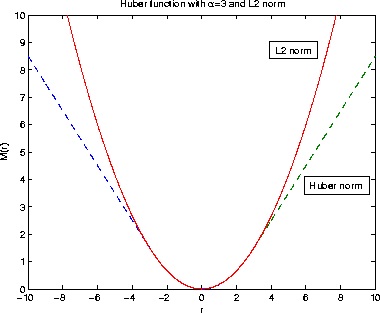
In this chapter, a hybrid $\ell^1/\ell^2$ error measure (or norm) proposed by Huber (1973) is presented:  

$$M_{\alpha}(r) = \left\{ \begin{array} {cc} \frac{r^2}{2\alph... ...t - \frac{\alpha}{2} & \alpha < \vert r\vert,\end{array}\right.$$ (1)

where $\alpha$ is the threshold between the $\ell^1$ and $\ell^2$ norm. The function $\sum_{i=1}^N\,M_{\alpha}(r_i)$ is called the ``Huber misfit function'', or Huber function for short. Figure shows the Huber norm as a function of the residual. It is smooth near zero residual, weights small residuals by mean square and treats large residuals with $\ell^1$. Because it is differentiable everywhere, it is reasonable to suppose that the Huber function is easier to minimize than $\ell^1$ while still robust against large residuals.

 

huber
Figure 1 Error measure with $\alpha=3$ proposed by Huber Huber (1973) (dash line) and the $\ell^2$norm (solid line).

Definition of the misfit via the Huber function results in a nonlinear optimization problem because any residual component r_i close to the threshold $\alpha$ can oscillate between the $\ell^1$ and $\ell^2$ norm. In the first section following this introduction, I propose solving the optimization problem with a quasi-Newton method called limited-memory BFGS Broyden (1969); Fletcher (1970); Goldfarb (1970); Nocedal (1980); Shanno (1970). In the second section, this method is tested to estimate the root mean square (rms) velocity (or slowness) of noisy common midpoint (CMP) and shot gathers for synthetic and field seismic data. There the Huber norm is compared with the $\ell^2$ norm with and without regularization.