

Next: Field data results
Up: Application of the Huber
Previous: Application of the Huber
Figure ![[*]](http://sepwww.stanford.edu/latex2html/cross_ref_motif.gif) displays the synthetic model. In
Figure
displays the synthetic model. In
Figure ![[*]](http://sepwww.stanford.edu/latex2html/cross_ref_motif.gif) a I show the ideal velocity space with five events at
different slownesses. In Figure
a I show the ideal velocity space with five events at
different slownesses. In Figure ![[*]](http://sepwww.stanford.edu/latex2html/cross_ref_motif.gif) b the five
corresponding hyperbolas in the CMP domain are shown. Finally in
Figure
b the five
corresponding hyperbolas in the CMP domain are shown. Finally in
Figure ![[*]](http://sepwww.stanford.edu/latex2html/cross_ref_motif.gif) c, four spikes are added to the CMP
gather in Figure
c, four spikes are added to the CMP
gather in Figure ![[*]](http://sepwww.stanford.edu/latex2html/cross_ref_motif.gif) b to make gaussian statistics
unsuitable. The energy of the four spikes is five times the energy of
the five hyperbolas.
Our goal is to find the velocity field
b to make gaussian statistics
unsuitable. The energy of the four spikes is five times the energy of
the five hyperbolas.
Our goal is to find the velocity field  that will
best fit a CMP gather
  via the HRT.
model
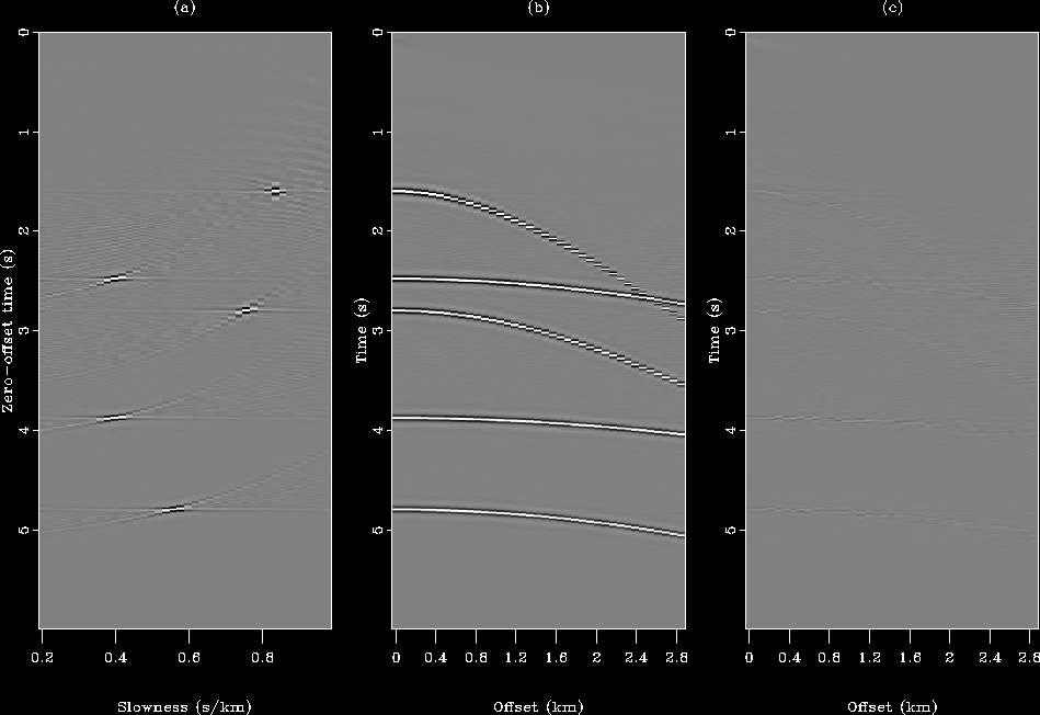
Figure 2 Synthetic data used
for the inversion. (a) The true velocity model represented in
slowness. (b) The noise-free input data used
for the inversion. (c) The same data but with noise
added (four spikes).


Figure ![[*]](http://sepwww.stanford.edu/latex2html/cross_ref_motif.gif) shows the result of the
inversion when the
shows the result of the
inversion when the  norm is used for the noise-free data.
On the left the velocity space is displayed with its five events.
The focusing is not perfect and some artifacts appear
Sacchi and Ulrych (1995).
The middle panel shows the remodeled data after inversion and
the right panel displays the residual (difference between
the input and remodeled data). I conclude that the inversion
reached a minimum since no coherent energy is left in the residual:
the data fitting is very good. Because the input data have
gaussian statistics, the performance of the least-squares inversion
was expected.
res-nospike-HUBER
Figure 3 Result
of the inversion with the  norm for the noise-free data.
(a) Inverted slowness field. (b) Remodeled data.
(c) Difference between the input (Figure
 ![[*]](http://sepwww.stanford.edu/latex2html/cross_ref_motif.gif) b)
and remodeled data.
b)
and remodeled data.


I now use the same inversion scheme with the  norm but with
the ``contaminated'' CMP gather (Figure
 ![[*]](http://sepwww.stanford.edu/latex2html/cross_ref_motif.gif) c).
Notice that no regularization was applied with the least-squares method.
The final result is shown in Figure
c).
Notice that no regularization was applied with the least-squares method.
The final result is shown in Figure ![[*]](http://sepwww.stanford.edu/latex2html/cross_ref_motif.gif) .
In this case, as expected, the
.
In this case, as expected, the  inversion
creates a number of artifacts both in the model and data space.
In the model space (Figure
 ![[*]](http://sepwww.stanford.edu/latex2html/cross_ref_motif.gif) a), the spikes are
mapped into curves whereas the hyperbola are mapped into nearly focused
points. In the data space, after remodeling (Figure
a), the spikes are
mapped into curves whereas the hyperbola are mapped into nearly focused
points. In the data space, after remodeling (Figure
![[*]](http://sepwww.stanford.edu/latex2html/cross_ref_motif.gif) b), spikes are not remodeled correctly
and are smearing on the neighboring traces.
In Figure
b), spikes are not remodeled correctly
and are smearing on the neighboring traces.
In Figure ![[*]](http://sepwww.stanford.edu/latex2html/cross_ref_motif.gif) I use least-squares
with a simple damping in the regularization. The model and data space
are cleaner but the difference between the input and the
remodeled data or residual is still large (comparing Figure
I use least-squares
with a simple damping in the regularization. The model and data space
are cleaner but the difference between the input and the
remodeled data or residual is still large (comparing Figure
![[*]](http://sepwww.stanford.edu/latex2html/cross_ref_motif.gif) c to Figure
c to Figure ![[*]](http://sepwww.stanford.edu/latex2html/cross_ref_motif.gif) c.)
In addition, artifacts in the inverted slowness
field and the reconstructed data can be seen.
c.)
In addition, artifacts in the inverted slowness
field and the reconstructed data can be seen.
res-spike-L2-HUBER
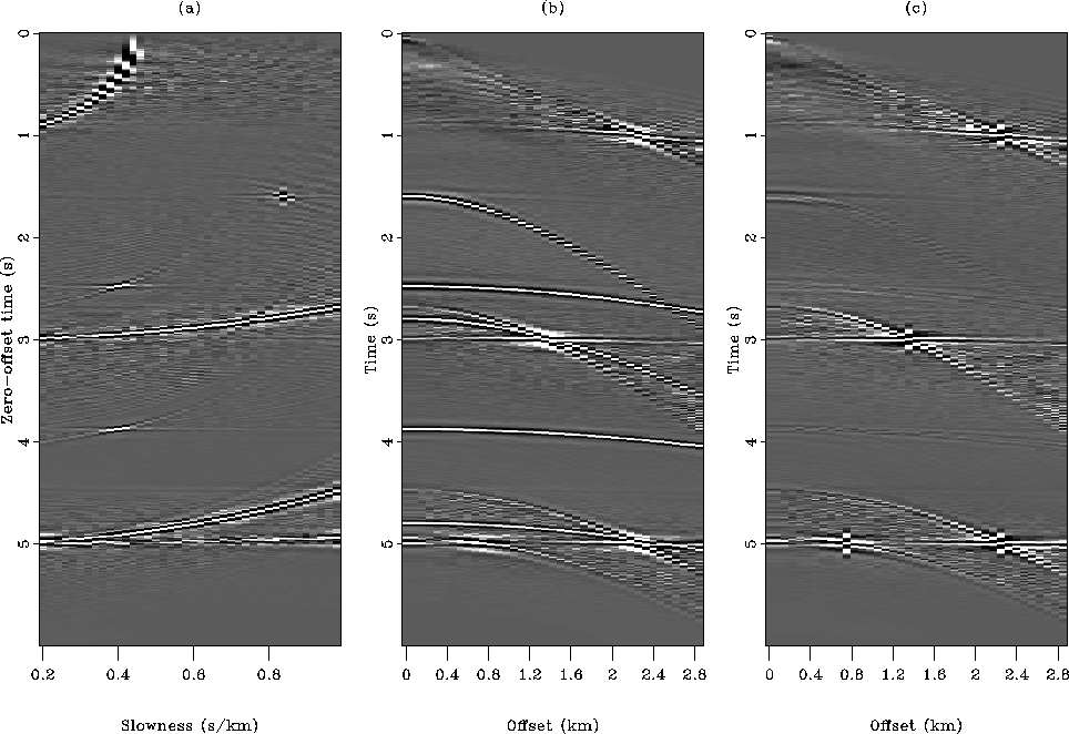
Figure 4 Result
of the inversion with the  norm for the data with
noise. (a) Inverted slowness field. (b) Remodeled data.
(c) Difference between the input (Figure
 ![[*]](http://sepwww.stanford.edu/latex2html/cross_ref_motif.gif) c)
and remodeled data. The four spikes create artifacts in both
inverted model and reconstructed data space.
c)
and remodeled data. The four spikes create artifacts in both
inverted model and reconstructed data space.


 res-spike-L2-reg-HUBER
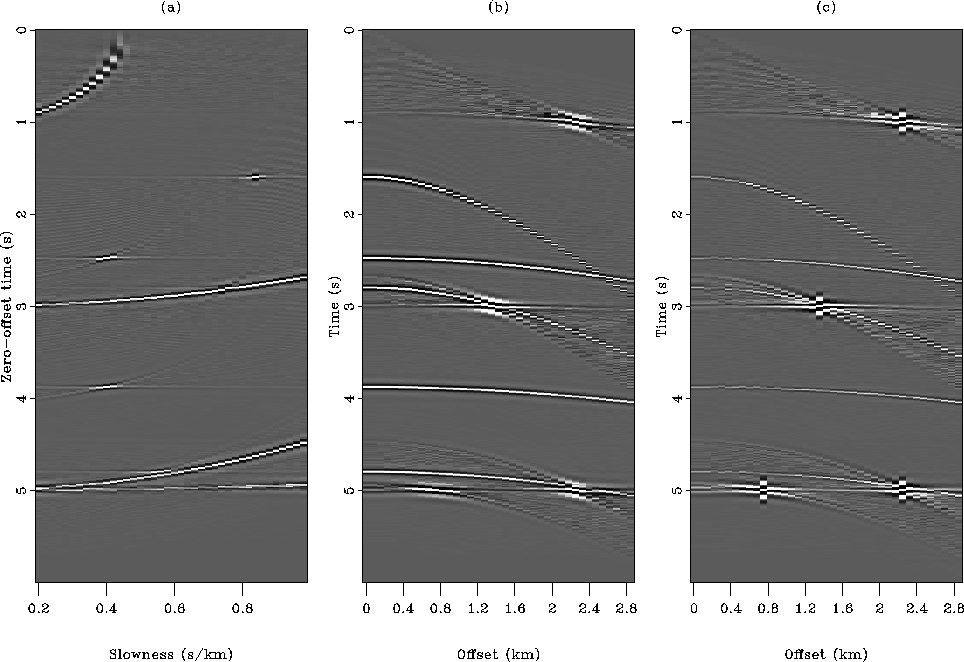
Figure 5 Result
of the inversion with the  norm with damping for the data with noise.
(a) Inverted slowness field. (b) Remodeled data.
(c) Difference between the input (Figure
 ![[*]](http://sepwww.stanford.edu/latex2html/cross_ref_motif.gif) c)
and remodeled data. The three panels are cleaner than in Figure
c)
and remodeled data. The three panels are cleaner than in Figure
![[*]](http://sepwww.stanford.edu/latex2html/cross_ref_motif.gif) but some artifacts remain, however.
but some artifacts remain, however.


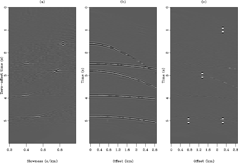
Figure ![[*]](http://sepwww.stanford.edu/latex2html/cross_ref_motif.gif) displays the result of the inversion
with the Huber norm. The outcome of the inversion is insensitive to
the spiky events, like a pure
displays the result of the inversion
with the Huber norm. The outcome of the inversion is insensitive to
the spiky events, like a pure  norm misfit function. The
residual (Figure
 ![[*]](http://sepwww.stanford.edu/latex2html/cross_ref_motif.gif) c) exhibits
the four spikes very clearly. This result demonstrates
that the proposed algorithm, although not specifically designed to minimize the
Huber function, converges to a satisfying solution. The next section shows
inversion results with noisy field data.
c) exhibits
the four spikes very clearly. This result demonstrates
that the proposed algorithm, although not specifically designed to minimize the
Huber function, converges to a satisfying solution. The next section shows
inversion results with noisy field data.
res-spike-HUBER
Figure 6 Result
of the robust inversion with the Huber norm for the data with
noise. (a) Inverted slowness field. (b) Remodeled data.
(c) Difference between the input (Figure ![[*]](http://sepwww.stanford.edu/latex2html/cross_ref_motif.gif) c)
and remodeled data. The Huber norm behaves like a pure
c)
and remodeled data. The Huber norm behaves like a pure
 norm since all artifacts have disappeared.


Next: Field data results
Up: Application of the Huber
Previous: Application of the Huber
Stanford Exploration Project
5/5/2005

![[*]](http://sepwww.stanford.edu/latex2html/cross_ref_motif.gif) displays the synthetic model. In
Figure
displays the synthetic model. In
Figure ![[*]](http://sepwww.stanford.edu/latex2html/cross_ref_motif.gif) a I show the ideal velocity space with five events at
different slownesses. In Figure
a I show the ideal velocity space with five events at
different slownesses. In Figure ![[*]](http://sepwww.stanford.edu/latex2html/cross_ref_motif.gif) b the five
corresponding hyperbolas in the CMP domain are shown. Finally in
Figure
b the five
corresponding hyperbolas in the CMP domain are shown. Finally in
Figure ![[*]](http://sepwww.stanford.edu/latex2html/cross_ref_motif.gif) c, four spikes are added to the CMP
gather in Figure
c, four spikes are added to the CMP
gather in Figure ![[*]](http://sepwww.stanford.edu/latex2html/cross_ref_motif.gif) b to make gaussian statistics
unsuitable. The energy of the four spikes is five times the energy of
the five hyperbolas.
Our goal is to find the velocity field
b to make gaussian statistics
unsuitable. The energy of the four spikes is five times the energy of
the five hyperbolas.
Our goal is to find the velocity field 
![[*]](http://sepwww.stanford.edu/latex2html/cross_ref_motif.gif) shows the result of the
inversion when the
shows the result of the
inversion when the ![]() norm is used for the noise-free data.
On the left the velocity space is displayed with its five events.
The focusing is not perfect and some artifacts appear
Sacchi and Ulrych (1995).
The middle panel shows the remodeled data after inversion and
the right panel displays the residual (difference between
the input and remodeled data). I conclude that the inversion
reached a minimum since no coherent energy is left in the residual:
the data fitting is very good. Because the input data have
gaussian statistics, the performance of the least-squares inversion
was expected.
norm is used for the noise-free data.
On the left the velocity space is displayed with its five events.
The focusing is not perfect and some artifacts appear
Sacchi and Ulrych (1995).
The middle panel shows the remodeled data after inversion and
the right panel displays the residual (difference between
the input and remodeled data). I conclude that the inversion
reached a minimum since no coherent energy is left in the residual:
the data fitting is very good. Because the input data have
gaussian statistics, the performance of the least-squares inversion
was expected.

![[*]](http://sepwww.stanford.edu/latex2html/cross_ref_motif.gif) b)
and remodeled data.
b)
and remodeled data.
![]() norm but with
the ``contaminated'' CMP gather (Figure
norm but with
the ``contaminated'' CMP gather (Figure ![[*]](http://sepwww.stanford.edu/latex2html/cross_ref_motif.gif) c).
Notice that no regularization was applied with the least-squares method.
The final result is shown in Figure
c).
Notice that no regularization was applied with the least-squares method.
The final result is shown in Figure ![[*]](http://sepwww.stanford.edu/latex2html/cross_ref_motif.gif) .
In this case, as expected, the
.
In this case, as expected, the ![]() inversion
creates a number of artifacts both in the model and data space.
In the model space (Figure
inversion
creates a number of artifacts both in the model and data space.
In the model space (Figure ![[*]](http://sepwww.stanford.edu/latex2html/cross_ref_motif.gif) a), the spikes are
mapped into curves whereas the hyperbola are mapped into nearly focused
points. In the data space, after remodeling (Figure
a), the spikes are
mapped into curves whereas the hyperbola are mapped into nearly focused
points. In the data space, after remodeling (Figure
![[*]](http://sepwww.stanford.edu/latex2html/cross_ref_motif.gif) b), spikes are not remodeled correctly
and are smearing on the neighboring traces.
In Figure
b), spikes are not remodeled correctly
and are smearing on the neighboring traces.
In Figure ![[*]](http://sepwww.stanford.edu/latex2html/cross_ref_motif.gif) I use least-squares
with a simple damping in the regularization. The model and data space
are cleaner but the difference between the input and the
remodeled data or residual is still large (comparing Figure
I use least-squares
with a simple damping in the regularization. The model and data space
are cleaner but the difference between the input and the
remodeled data or residual is still large (comparing Figure
![[*]](http://sepwww.stanford.edu/latex2html/cross_ref_motif.gif) c to Figure
c to Figure ![[*]](http://sepwww.stanford.edu/latex2html/cross_ref_motif.gif) c.)
In addition, artifacts in the inverted slowness
field and the reconstructed data can be seen.
c.)
In addition, artifacts in the inverted slowness
field and the reconstructed data can be seen.

![[*]](http://sepwww.stanford.edu/latex2html/cross_ref_motif.gif) c)
and remodeled data. The four spikes create artifacts in both
inverted model and reconstructed data space.
c)
and remodeled data. The four spikes create artifacts in both
inverted model and reconstructed data space.

![[*]](http://sepwww.stanford.edu/latex2html/cross_ref_motif.gif) c)
and remodeled data. The three panels are cleaner than in Figure
c)
and remodeled data. The three panels are cleaner than in Figure
![[*]](http://sepwww.stanford.edu/latex2html/cross_ref_motif.gif) but some artifacts remain, however.
but some artifacts remain, however.
![[*]](http://sepwww.stanford.edu/latex2html/cross_ref_motif.gif) displays the result of the inversion
with the Huber norm. The outcome of the inversion is insensitive to
the spiky events, like a pure
displays the result of the inversion
with the Huber norm. The outcome of the inversion is insensitive to
the spiky events, like a pure ![]() norm misfit function. The
residual (Figure
norm misfit function. The
residual (Figure ![[*]](http://sepwww.stanford.edu/latex2html/cross_ref_motif.gif) c) exhibits
the four spikes very clearly. This result demonstrates
that the proposed algorithm, although not specifically designed to minimize the
Huber function, converges to a satisfying solution. The next section shows
inversion results with noisy field data.
c) exhibits
the four spikes very clearly. This result demonstrates
that the proposed algorithm, although not specifically designed to minimize the
Huber function, converges to a satisfying solution. The next section shows
inversion results with noisy field data.

![[*]](http://sepwww.stanford.edu/latex2html/cross_ref_motif.gif) c)
and remodeled data. The Huber norm behaves like a pure
c)
and remodeled data. The Huber norm behaves like a pure