Next: Conclusion
Up: Application of the Huber
Previous: Synthetic data results
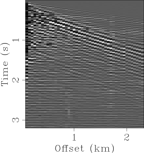
The proposed algorithm is now tested on a field data example. For this
purpose, a shot gather from a land-data survey in the Middle East is selected. The
trajectories of the events in Figure ![[*]](http://sepwww.stanford.edu/latex2html/cross_ref_motif.gif) look ``hyperbolic''
enough to be inverted with our method. Note that in theory,
the data should be sorted into CMP gathers before doing the inversion.
This dataset is particularly interesting because it has amplitude
anomalies at short offset and a low velocity coherent noise that is
probably due to guided energy in the near-surface. I could attenuate
the amplitude anomalies by applying an Automatic Gain Control (AGC) on the
data before inversion. A better approach is by weighting the residual
with a function mimicking AGC.
look ``hyperbolic''
enough to be inverted with our method. Note that in theory,
the data should be sorted into CMP gathers before doing the inversion.
This dataset is particularly interesting because it has amplitude
anomalies at short offset and a low velocity coherent noise that is
probably due to guided energy in the near-surface. I could attenuate
the amplitude anomalies by applying an Automatic Gain Control (AGC) on the
data before inversion. A better approach is by weighting the residual
with a function mimicking AGC.
model2
Figure 7 The field data used
for the inversion. Notice the amplitude anomalies at near offset and
the time shift near offset 2 km.
|
|  |


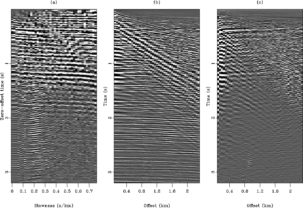
This gather is first inverted with the  norm without regularization
(Figure ). The left panel displays the
velocity domain obtained after the least-squares inversion. The main velocity
event is masked with horizontal stripes coming from the short-offset
amplitude anomalies. The reconstructed data (middle panel) show
spurious noise at large offset and other inversion artifacts.
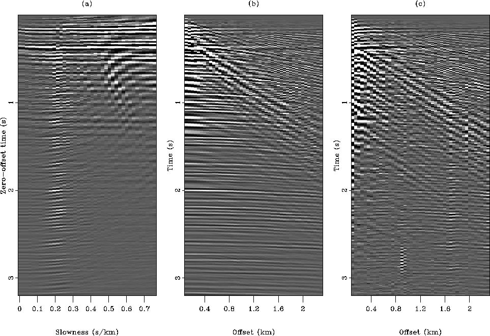
I now show in Figure the result
of the damped least-squares. The inverted slowness field is much
cleaner, but the horizontal stripes remain. We also have the
same velocity from the top to the bottom of Figure
a. This shows that the data are
contaminated with multiples generated in the near surface.
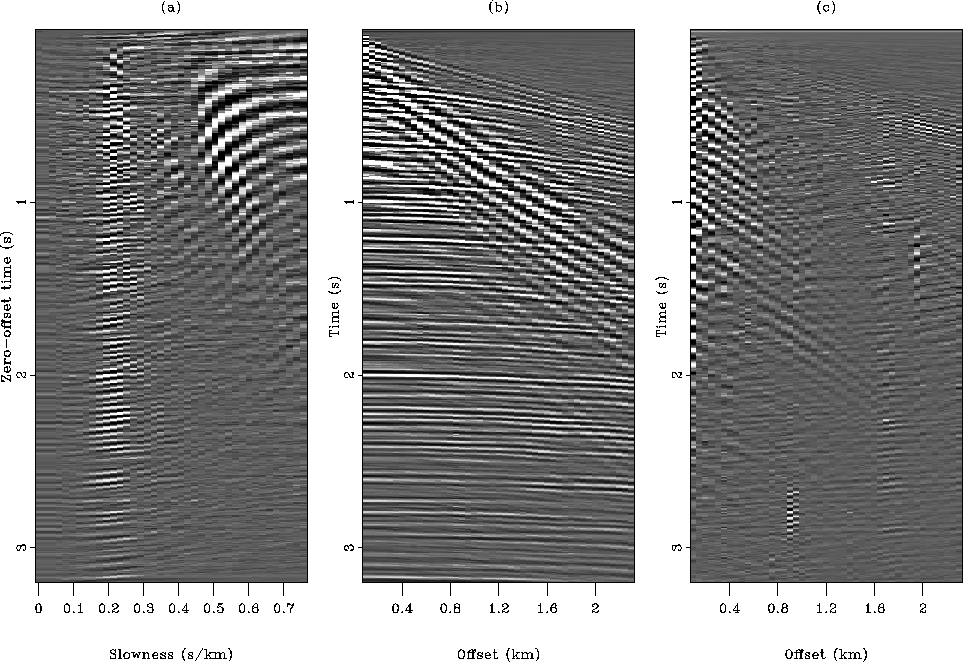
Figure displays the inversion result
with the Huber norm and demonstrates the robustness of this method.
A very well focused velocity corridor is obtained as opposed to the
result in Figure a. In addition,
the horizontal stripes have disappeared.
norm without regularization
(Figure ). The left panel displays the
velocity domain obtained after the least-squares inversion. The main velocity
event is masked with horizontal stripes coming from the short-offset
amplitude anomalies. The reconstructed data (middle panel) show
spurious noise at large offset and other inversion artifacts.
I now show in Figure the result
of the damped least-squares. The inverted slowness field is much
cleaner, but the horizontal stripes remain. We also have the
same velocity from the top to the bottom of Figure
a. This shows that the data are
contaminated with multiples generated in the near surface.
Figure displays the inversion result
with the Huber norm and demonstrates the robustness of this method.
A very well focused velocity corridor is obtained as opposed to the
result in Figure a. In addition,
the horizontal stripes have disappeared.
The synthetic and field data examples demonstrate that
the Huber norm can be an efficient alternative to the
norm when outliers (or non-gaussian noise) are present
in the data.
res-wz08-L2-HUBER
Figure 8 The result
of the inversion with the norm for the field data.
(a) Inverted slowness field. (b) Remodeled data.
(c) Difference between the input (Figure )
and remodeled data. The horizontal stripes in the velocity panel
are created by the amplitude anomalies at short offsets.
res-wz08-L2-reg-HUBER
Figure 9 The result
of the inversion with the norm and regularization for the field data.
(a) Inverted slowness field. (b) Remodeled data.
(c) Difference between the input (Figure )
and remodeled data. The model is much cleaner that in Figure
a, but the horizontal events remain.
res-wz08-0.082-HUBER
Figure 10 The result
of the robust inversion with the Huber norm for the field data.
(a) Inverted slowness field. (b) Remodeled data.
(c) Difference between the input (Figure )
and remodeled data.
Next: Conclusion
Up: Application of the Huber
Previous: Synthetic data results
Stanford Exploration Project
5/5/2005