


Next: Linearized image perturbations
Up: Wave-equation migration velocity analysis
Previous: Wave-equation migration velocity analysis
Imaging by wavefield extrapolation (WE) is based on recursive
continuation of wavefields  from a given depth level
to the next by means of an extrapolation operator
from a given depth level
to the next by means of an extrapolation operator  .At every extrapolation step, we can write that
|  |
(92) |
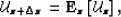
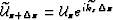
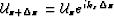
where  is the wavefield at the top of the slab, and
 is the wavefield at the bottom of the slab.
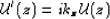
The operator involves a spatially-dependent
phase shift described by:
is the wavefield at the bottom of the slab.
The operator involves a spatially-dependent
phase shift described by:
|  |
(93) |
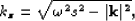
where  represents the depth wavenumber, and
 the wavefield extrapolation depth step.
The relation (
the wavefield extrapolation depth step.
The relation (![[*]](http://sepwww.stanford.edu/latex2html/cross_ref_motif.gif) )
corresponds to the analytical solution of
the differential equation
)
corresponds to the analytical solution of
the differential equation
|  |
(94) |
which describes depth extrapolation of monochromatic
plane waves (24).
The ' sign represents a derivative with respect to the
depth z.
The depth wavenumber is given by the one-way wave equation,
also known as the single square root (SSR) equation
|  |
(95) |
where  is the temporal frequency,
s is the laterally variable slowness of the medium, and
is the temporal frequency,
s is the laterally variable slowness of the medium, and
 is the horizontal wavenumber.
I use the laterally variable s and the horizontal wavenumber
in SSR just for conciseness,
although such a notation not mathematically correct in laterally
varying media.
is the horizontal wavenumber.
I use the laterally variable s and the horizontal wavenumber
in SSR just for conciseness,
although such a notation not mathematically correct in laterally
varying media.
Since downward continuation by Fourier-domain
phase shift can be applied for slowness
models that only vary with depth, we need to split the operator
into two parts: a constant slowness continuation operator
applied in the  domain, which accounts for the propagation
in depth, and a screen operator applied in the
domain, which accounts for the propagation
in depth, and a screen operator applied in the
 domain, which accounts for the wavefield perturbations
due to the lateral slowness variations.
In essence, we approximate the vertical wavenumber with its constant
slowness counterpart
domain, which accounts for the wavefield perturbations
due to the lateral slowness variations.
In essence, we approximate the vertical wavenumber with its constant
slowness counterpart  , corrected by a term describing the spatial
variability of the slowness function (81).
, corrected by a term describing the spatial
variability of the slowness function (81).
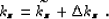
Furthermore, we can separate the depth wavenumber into two components,
one which corresponds to the background medium  and
one which corresponds to a perturbation of the medium:
and
one which corresponds to a perturbation of the medium:
|  |
(96) |
In a first-order approximation, we can relate those two depth wavenumbers
by a Taylor series expansion:
&& + . d
d s |_s=ss - s
&& + s^2 s^2 - |k|^2 s - s,
where
 is the slowness corresponding to the perturbed medium, and
 is the background slowness.
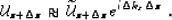
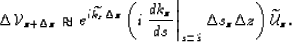
Within any depth slab, we can extrapolate the wavefield
from the top either in the perturbed or in the background medium.
The wavefields at the bottom of the slab,
 and
and
 are related by the relation
|  |
(97) |
rytov.w is a direct statement of the Rytov approximation
(56), since
the wavefields at the bottom of the slab correspond to different
phase shifts related by a linear equation.
The wavefield perturbation  at the bottom of the slab
is obtained by subtracting
the background wavefield
at the bottom of the slab
is obtained by subtracting
the background wavefield  from the perturbed wavefield :
&& -
&& e^i-1
&& e^i e^i . d
d s |_s=ss -1 ,
where  is the perturbation between the correct and
the background slownesses at depth z.
is the perturbation between the correct and
the background slownesses at depth z.
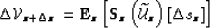
In operator form we can write
| 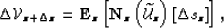 |
(98) |
where  represents the downward continuation operator at depth z,
and
represents the downward continuation operator at depth z,
and  represents the Rytov scattering operator which is
dependent on the background wavefield
represents the Rytov scattering operator which is
dependent on the background wavefield  and the
slowness perturbation
and the
slowness perturbation  at that depth level:
|  |
(99) |
In this approximation, we assume that the scattered wavefield is generated
only by the background wavefield and we ignore all multi-scattering effects.
For the Born approximation
(56), we further assume that the wavefield
differences are small, such we can linearize the exponential
according to the relation  .
With this new approximation, the expression for the
downward-continued scattered wavefield becomes:
.
With this new approximation, the expression for the
downward-continued scattered wavefield becomes:
|  |
(100) |
In operator form, we can write the scattered wavefield at z as
|  |
(101) |
where
represents the downward continuation operator at depth z, and
 represents the Born scattering operator which is dependent
on the background wavefield and operates on the slowness
perturbation at that depth level.
represents the Born scattering operator which is dependent
on the background wavefield and operates on the slowness
perturbation at that depth level.
The linear scattering operator  is a mixed-domain operator similar
to the extrapolation operator . This operator depends on the
background wavefield and background slowness by the expression:
is a mixed-domain operator similar
to the extrapolation operator . This operator depends on the
background wavefield and background slowness by the expression:
| 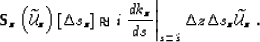 |
(102) |
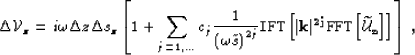
In practice, we can implement the scattering operator described
by born.op in different ways.
One option is to implement the Born operator born.op
in the space domain using an expansion
(50) like
|  |
(103) |
In practice, the summation of the terms in born.exp
involves forward and inverse Fast
Fourier Transforms (FFT and IFT)
and multiplication in the
space domain with the spatially variable  :
:
|  |
(104) |
where  Another option is to implement the Born operator born.op
in the Fourier domain relative to the constant reference slowness in
any individual slab. In this case, we can write
Another option is to implement the Born operator born.op
in the Fourier domain relative to the constant reference slowness in
any individual slab. In this case, we can write
| 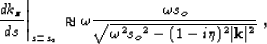 |
(105) |
where  as a damping parameter which avoids division by zero
(48).
In practice, the implementation of born.sqr
involves forward and inverse Fast
Fourier Transforms (FFT and IFT):
as a damping parameter which avoids division by zero
(48).
In practice, the implementation of born.sqr
involves forward and inverse Fast
Fourier Transforms (FFT and IFT):
| 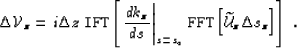 |
(106) |
Next: Linearized image perturbations
Up: Wave-equation migration velocity analysis
Previous: Wave-equation migration velocity analysis
Stanford Exploration Project
11/4/2004