


The original data set was computed with a typical marine off-end recording geometry. Preliminary studies of the data demonstrated that in some areas the complex overburden causes events to be reflected with negative reflection angle (i.e. the source and receiver wavepaths cross before reaching the reflector). To avoid losing these events I applied the reciprocity principle and created a split-spread data set from the original off-end data set. This modification of the data set enabled us to compute symmetric ADCIGs that are easier to visually analyze than the typical one-sided ADCIGs obtained from marine data. Therefore, I display the symmetric ADCIGs in SIG.srm and SIG.ang08-SIG.ang12. Doubling the dataset also doubles the computational cost of the WEMVA process.
 |
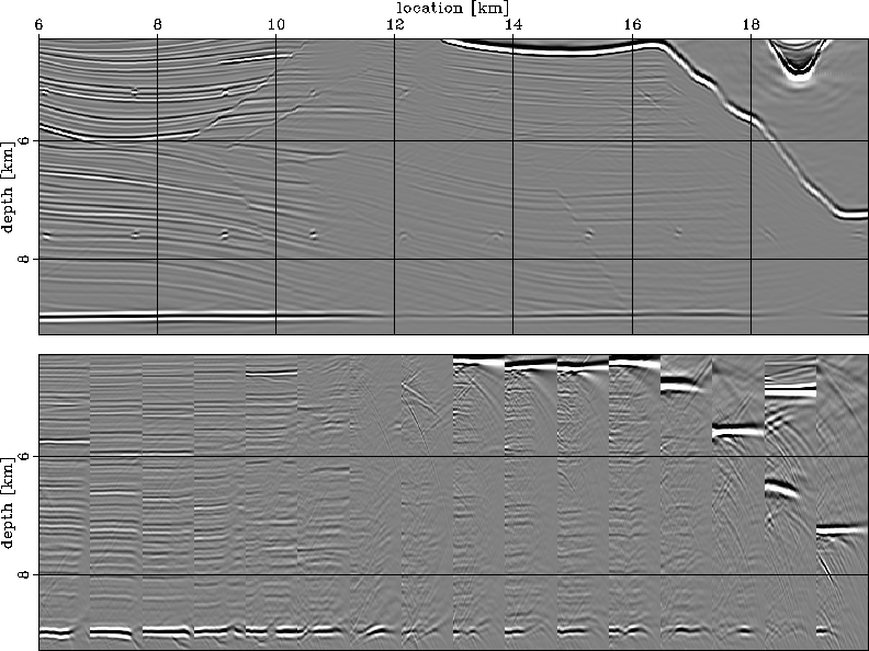
SIG.imgC shows the migrated image using the correct slowness model. The top panel shows the zero offset of the prestack migrated image, and the bottom panel depicts ADCIGs at equally spaced locations in the image. Each ADCIG corresponds roughly to the location right above it.
 |
This image highlights several characteristics of this model that make it a challenge for migration velocity analysis. Most of them are related to the complicated wavepaths in the subsurface under rough salt bodies. First, the angular coverage under salt (x>11 km) is much smaller than in the sedimentary section uncovered by salt (x<11 km). Second, the subsalt region is marked by many illumination gaps or shadow zones, the most striking being located at x=12 and x=19 km. The main consequence is that velocity analysis in the poorly illuminated areas are much less constrained than in the well illuminated zones, as will become apparent later on in this example.
I begin by migrating the data with the background slowness (SIG.img1). As before, the top panel shows the zero offset of the prestack migrated image, and the bottom panel depicts angle-domain common image gathers at equally spaced locations in the image. Since the migration velocity is incorrect, the image is defocused and the angle gathers show significant moveout. Furthermore, the diffractors at depths z=7.5 km, and the fault at x=15 km are defocused.
 |
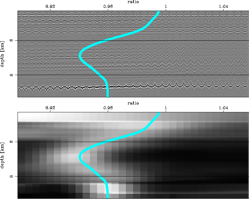
I run prestack Stolt residual migration storm
for various values of a velocity
ratio parameter ![]() between 0.9
and 1.6, which ensures that a
fairly wide range of the velocity space is spanned.
Although residual migration operates on the entire
image globally, for display purposes I extract
one gather at x=10 km.
SIG.srm shows at the top the
ADCIGs for all velocity ratios and at the bottom
the semblance panels computed from the ADCIGs.
I pick the maximum semblance at all locations and
all depths (SIG.pck), together
with an estimate of the reliability of every picked
value which I use as a weighting function on the
data residuals during inversion.
between 0.9
and 1.6, which ensures that a
fairly wide range of the velocity space is spanned.
Although residual migration operates on the entire
image globally, for display purposes I extract
one gather at x=10 km.
SIG.srm shows at the top the
ADCIGs for all velocity ratios and at the bottom
the semblance panels computed from the ADCIGs.
I pick the maximum semblance at all locations and
all depths (SIG.pck), together
with an estimate of the reliability of every picked
value which I use as a weighting function on the
data residuals during inversion.
 |
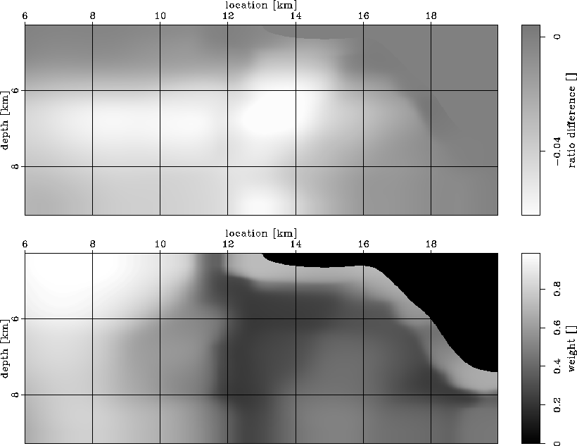 |
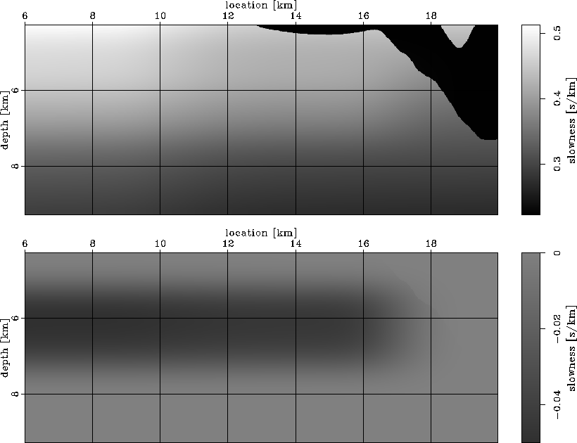
Based on the picked velocity ratio, I compute the linearized differential image perturbation, as described in the preceding sections. Next, I invert for the slowness perturbation depicted in the bottom panel of SIG.dsl. For comparison, the top panel of SIG.dsl shows the correct slowness perturbation relative to the correct slowness. I can clearly see the effects of different angular coverage in the subsurface: at x<11 km, the inverted slowness perturbation is better constrained vertically than it is at x>11 km.
 |
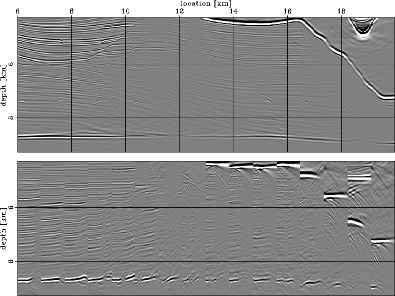
Finally, I update the slowness model and remigrate the data (SIG.img2). As before, the top panel shows the zero offset of the prestack migrated image, and the bottom panel depicts angle-domain common image gathers at equally spaced locations in the image. With this updated velocity, the reflectors have been repositioned to their correct location, the diffractors at z=7.5 km are focused and the ADCIGs are flatter than in the background image, indicating that the slowness update has improved the quality of the migrated image.
 |
SIG.ang08-SIG.ang12
show a more detailed analysis of the results of the
inversion displayed as ADCIGs at various locations
in the image.
In each figure, the panels correspond
to migration with the correct slowness (left), the
background slowness (center),
and the updated slowness (right).
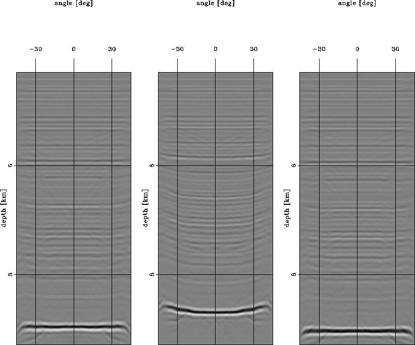
SIG.ang08 corresponds to an ADCIG at
x=8 km, in the region which is well illuminated.
The angle gathers are clean, with clearly
identifiable moveouts that are corrected after inversion.
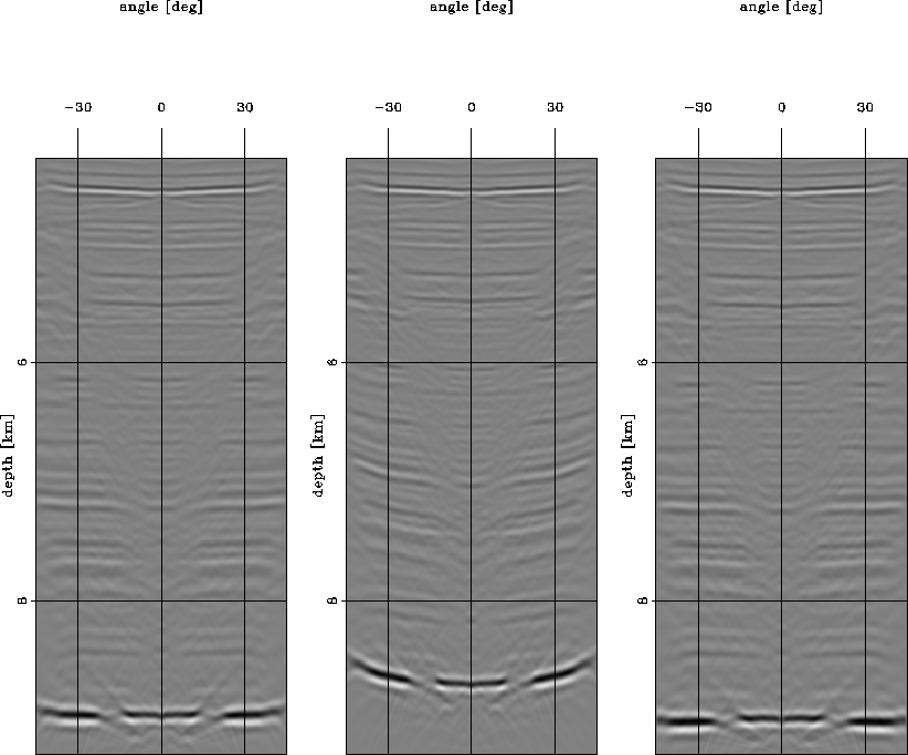
SIG.ang10 corresponds to an ADCIG at
x=10 km, in the region with illumination gaps,
clearly visible on the strong reflector at z=9 km
at a scattering angle of about ![]() .The gaps are preserved in the ADCIG from the image migrated
with the background slowness, but the moveouts are still
easy to identify and correct.
Finally, SIG.ang12 corresponds to an ADCIG at
x=12 km, in a region which is poorly illuminated.
In this case, the ADCIG is much noisier
and the moveouts are
harder to identify and measure. This region also
corresponds to the lowest reliability, as indicated by
the low weight of the picks (SIG.pck).
The gathers in this region
contribute less to the inversion and the resulting
slowness perturbation is mainly controlled by
regularization. Despite the noisier gathers, after
slowness update and re-migration I recover an image
reasonably similar to the one obtained by
migration with the correct slowness.
.The gaps are preserved in the ADCIG from the image migrated
with the background slowness, but the moveouts are still
easy to identify and correct.
Finally, SIG.ang12 corresponds to an ADCIG at
x=12 km, in a region which is poorly illuminated.
In this case, the ADCIG is much noisier
and the moveouts are
harder to identify and measure. This region also
corresponds to the lowest reliability, as indicated by
the low weight of the picks (SIG.pck).
The gathers in this region
contribute less to the inversion and the resulting
slowness perturbation is mainly controlled by
regularization. Despite the noisier gathers, after
slowness update and re-migration I recover an image
reasonably similar to the one obtained by
migration with the correct slowness.
A simple visual comparison of the middle panels with the right and left panels in SIG.ang08-SIG.ang12 unequivocally demonstrates that the WEMVA method overcomes the limitations related to the linearization of the wave equation by using the first-order Born approximation. The images obtained using the initial velocity model (middle panels) are vertically shifted by several wavelengths with respect to the images obtained using the true velocity (left panels) and the estimated velocity (right panels). If the Born approximation were a limiting factor for the magnitude and spatial extent of the velocity errors that could be estimated with the WEMVA method, I would have been unable to estimate a velocity perturbation sufficient to improve the ADCIGs from the middle panels to the right panels.
 |


Angle-domain common image gathers at x=8 km.
Panels (a) and (c) correspond to
Cartesian coordinates, and
panels (b) and (d) correspond to
ray coordinates.
Velocity model with an overlay of the
ray coordinate system initiated by a <
source at the surface (a);
image obtained by downward continuation in
Cartesian coordinates with the
![]() equation (c);
velocity model with an overlay of the
ray coordinate system (b);
image obtained by wavefield extrapolation in
ray coordinates with the
equation (c);
velocity model with an overlay of the
ray coordinate system (b);
image obtained by wavefield extrapolation in
ray coordinates with the
![]() equation (d).<3181>>
equation (d).<3181>>
 |
Angle-domain common image gathers at x=10 km.
Panels (a) and (c) correspond to
Cartesian coordinates, and
panels (b) and (d) correspond to
ray coordinates.
Velocity model with an overlay of the
ray coordinate system initiated by a <
source at the surface (a);
image obtained by downward continuation in
Cartesian coordinates with the
![]() equation (c);
velocity model with an overlay of the
ray coordinate system (b);
image obtained by wavefield extrapolation in
ray coordinates with the
equation (c);
velocity model with an overlay of the
ray coordinate system (b);
image obtained by wavefield extrapolation in
ray coordinates with the
![]() equation (d).<3185>>
equation (d).<3185>>
 |
Angle-domain common image gathers at x=12 km.
Panels (a) and (c) correspond to
Cartesian coordinates, and
panels (b) and (d) correspond to
ray coordinates.
Velocity model with an overlay of the
ray coordinate system initiated by a <
source at the surface (a);
image obtained by downward continuation in
Cartesian coordinates with the
![]() equation (c);
velocity model with an overlay of the
ray coordinate system (b);
image obtained by wavefield extrapolation in
ray coordinates with the
equation (c);
velocity model with an overlay of the
ray coordinate system (b);
image obtained by wavefield extrapolation in
ray coordinates with the
![]() equation (d).<3189>>
equation (d).<3189>>