Regularization

Our velocity model is sampled in $1 {\rm km}$ in both depth and x position. Our total number of model points is approximately seven times our number of data points. As a result our model is significantly undeterdetermined. There are several ways to deal with the problem. One solution would be to decrease the number of grid points by sampling differently (coarser regular sampling or some type of irregular sampling). We can improve the situation by back propagating along fatter rays or we can add some type of regularization operator. Potentially the most interesting, and the one chosen for this paper is to add a regularization operator.

The typical choice for a regularization operator is an isotropic roughner. This will tend to fill undetermined portions of the model with isotropic blobs. In many cases this is unrealistic. Generally velocity follows structure and our structure is laid down as a series of layers that are later deformed by tectonic processes. A better choice for our regularization operator is something that tends to create features that follow structure. Clapp (2001) showed that this can improve the velocity estimate for oil exploration targets. Our regularization operator becomes a steering filter, a non-stationary filter which tends to smooth along some predefined dip map. 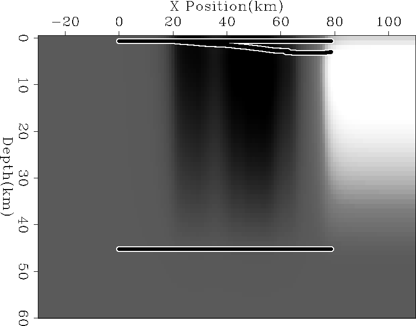In this case we used three reflectors to build the dip map from: the surface, a basement reflector, and the Moho. We measure the dip along each reflector and then interpolate between them. Figure  shows the dip field overlain by the reflectors.

 

dips Figure 4 The dip field and reflectors used to construct the steering filter operator. The upward dip on the right edge is due to continuing the dip present at the edge of the reflectors.

We want to smooth the slowness model, not the change in slowness that we are inverting for. As a result our regularization fitting goal becomes

$$\bf 0\approx \bf A( {\bf s_0} + \bf \Delta s) ,$$ (3)

where $\bf s_{0}$ is the initial slowness and $\bf A$is our steering filter. This problem converges quite slowly. As a result we precondition the model using the inverse of our regularization operator Claerbout (1999). Our final set of fitting goals become

$$\begin{eqnarray} \bf \Delta t&\approx&\bf T_{0} \bf A^{-1}\bf p \\ \bf 0&\approx&\epsilon \bf p\nonumber ,\end{eqnarray}$$ (4)

where $\bf p$ is the preconditioned variable and $\epsilon$ is a twiddle parameter controlling the amount of smoothing. Figure  shows the resulting change in velocity and the updated velocity model. Note how the basin structure that has now appears in the model.

 

vel1
Figure 5 The left panel shows the updated velocity model. The right panel is the change in velocity resulting from 120 iterations of fitting goals (4).