TOMOGRAPHY

We linearize the tomography problem around an initial slowness model $\bf s_{0}$. Rays are traced through the model based on the recorded arrival direction. The length of the ray segments through each model cell form the basis of the tomography operator $\bf T_{0}$.Figure   show the rays forming $\bf T_{0}$overlying the initial velocity model. Note that we have decent angular coverage.

 

rays Figure 3 The rays forming 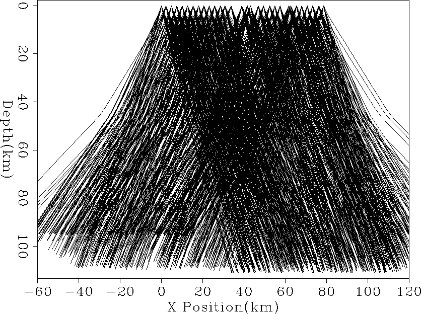$\bf T_{0}$overlying the initial velocity model.

For this experiment we are limiting ourselves to a 2-D earth model. As shown in Figure , our selected set of earthquakes are approximately oriented along the receiver line. For this experiment we assume constant velocity out of plane. We do 2-D ray tracing and then correct all lengths by

$$l_{{\rm new}} = \frac{l_{{\rm old}}}{ \Vert \cos (\phi)\Vert},$$ (1)

where $l_{{\rm old}}$ is the old ray length, $l_{{\rm new}}$is the updated ray length and $\phi$ is the azimuth direction of the earthquake.

Each arrival time also has a variance associated with it. The inverse of these variances form a noise covariance operator $\bf W_{{\rm 0}}$ for the inversion. We invert for the change in slowness $\bf \Delta s$ by minimizing the fitting goal,

$$\bf 0\approx \bf W_{{\rm 0}} ( \bf \Delta t- \bf T_{0} \bf \Delta s).$$ (2)

 

• Regularization