CGG Green Canyon IV 3-D Data

In 2003, CGG donated a large portion of a 161-block speculative seismic survey it acquired in the Green Canyon region of the Gulf of Mexico. The data were acquired in the transition zone between the edge of the Continental Shelf and the Sigsbee escarpment which signals the edge of the abyssal plain. Geologically, the Green Canyon region is characterized by sedimentary ``minibasins'' interrupted by complex salt bodies AAPG (1998).

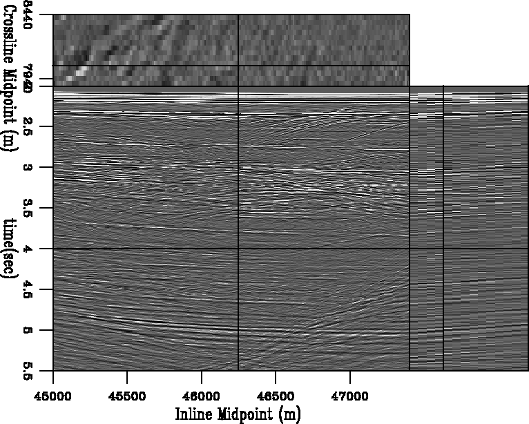
CGG's 3-D data were acquired by a ship sailing east-to-west, in the strike direction relative to the dominant geologic dip. The subset of the data that I process in this paper contains fairly significant crossline dip ($\gt 3^{\circ}$)in most places. Figure 3 shows a stacked section of the subset, which contains 192 midpoints inline and 14 midpoints crossline. The stacked section includes contributions from two adjacent sail lines, the geometries of which are illustrated in Figure 4.

 

stackraw3d.gc3d
Figure 3 Stacked section of subset of Green Canyon IV 3-D dataset.

 

feather
Figure 4 Acquisition geometry for two sail lines contributing to subset shown in Figure 3. ``S'' symbols illustrate source positions. ``M'' and ``F'' symbols illustrate the medium- and far-offset receivers, respectively, on each of the boat's four streamers. The nominal sail line spacing is 300 meters, although it varies considerably in this case from about 200 to 500 meters. The subset processed in this section contains shot records from about 40,000 to 50,000 meters inline location. Cable feathering in this zone is present, though not severe. The two sail lines overlap to some extent, which reduces the number of crossline midpoint locations from these two sail lines to 14 from 16 over the subset.

The subset shown in Figure 3 is situated in a sedimentary minibasin, with strong reflections visible at a two-way traveltime of well over 5 seconds. Thanks to a strong velocity gradient and the sparse offset sampling, surface-related multiples are largely absent from the stacked section. Still, as we shall see, the multiples are fairly strong in the prestack data and inhibit prestack amplitude analysis. The section exhibits moderate reflector dip - an anticlinal structure in the inline direction and effectively constant crossline dip of several degrees.

The acquisition ship sailed quite fast, with a flip-flop source interval of 37.5 meters, and an interval of 75 meters between like sources. The fast ship speed leads to reduced resolution along the inline offset axis: for an 8100-meter cable with receiver group spacing of 25 meters, the nominal CMP fold is only 54, implying a nominal inline offset spacing of 150 meters. Figure 5 illustrates the sparse sampling of the inline offset axis. While the nominal inline offset bin size of 150 meters ensures that all bins will contain a live trace, such sparsity will greatly inhibit the estimation of reasonable stacking velocities and create ``checkerboard'' artifacts in the shallow portions of a stacked image.

 

sparse.gc3d Figure 5 Illustration of sparsity of inline offset axis of CGG Green Canyon IV data. Grid represents nominal bin size of 150x12.5 meters. Black dots correspond to trace locations.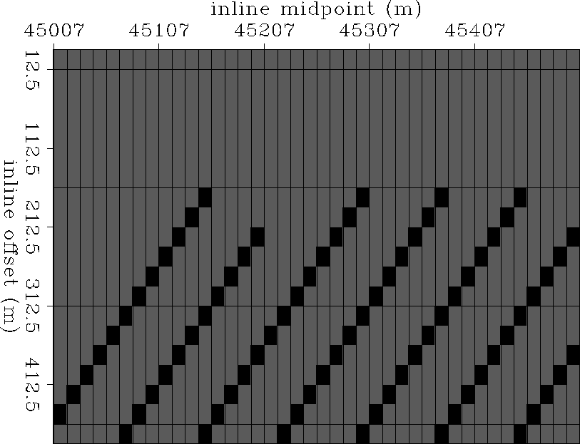

Therefore, in my processing of this dataset, I use an offset bin spacing of 25 meters. While this fine sampling better honors the physics of the experiment, it leads to a fivefold increase in empty bins. Moreover, although I have cast LSJIMP primarily as a wavefield separation algorithm, recall that one major motivation of integrating multiples and primaries is to use the multiples as a constraint on the primaries in zones where we do not record data. Multiples sample reflectors more finely in reflection angle/offset than do primaries. Moreover, the regularization strategies discussed earlier provide the infrastructure to exploit the inherent multiplicity of signal within an image and between multiple and primary images. Although designed to separate signal and noise, these same strategies also prove adept at interpolating signal in missing traces.

Stacking velocities were computed by a conventional velocity scan, coupled with maximum amplitude autopicking and local weighted (stack power) mean smoothing. The residual weight, simply zero for missing traces, but one elsewhere, is particularly important to achieve a successful LSJIMP result.