 |
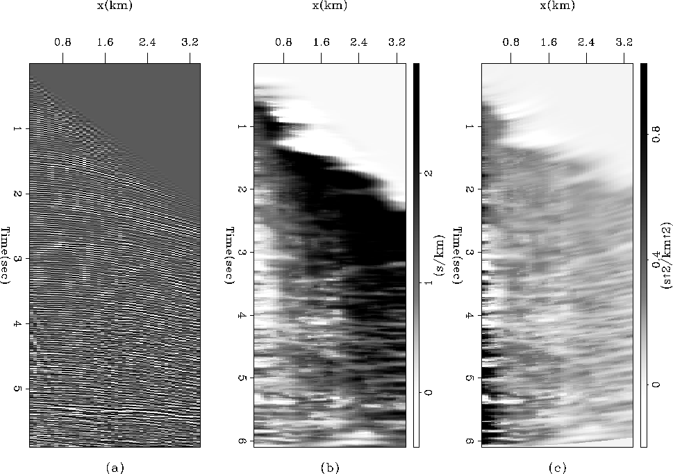
Figure 4 (a) Shot gather 14 with AGC, (b) estimated local dip, and (c) estimated s2 after NMO correction of 2.5 km/s.
Once the method was shown to work on an idealized synthetic case, we tested it on some real shot gathers to see how robust the method is when working with real data and the problems inherent with them. Theoretically, CMP gathers should be used for this analysis, however we have decided to use the Yilmaz-Cumro shot gathers to test our method. The 40 shots in the dataset provide varying data quality and numerous challenges, which will thoroughly test the robustness of our method.
Figure 4a shows shot 14 from the Yilmaz-Cumro shot gather dataset. The shot is a fairly clean record consisting of many hyperbolic events that should give a good velocity estimate. Examining Figure 4b, which shows the dip estimate, there are areas at the top of the profile that have negative dips. These result from the low velocity direct arrivals visible in the data; the dip estimator picks the aliased energy for its dip estimate. In the same area in Figure 4c the negative dip estimates result in a negative estimate for the value of s2. Although this is an undesirable result, these values will be accounted for and disregarded by the median stacking routine. The estimate of s2 has had an NMO correction applied to it with an arbitrary velocity of 2.5 km/s. Although most of the hyperbolas are not well flattened, synthetic example results show that this has little effect on the output from the median stack.
 |
The estimated RMS velocity profile created by median stacking Figure 4c is shown in Figure 5. At early times the estimate varies due to a lack of information from large offsets required to help constrain the velocity. For this reason the begining of the estimate is erased and replaced by extending a reasonable value back to time zero. The estimate also fluctuates at later times in the record, because the data become noisier, causing dip estimates to become unstable.
|
14velocity
Figure 5 Estimated RMS velocity profile for the data in Figure 4. | 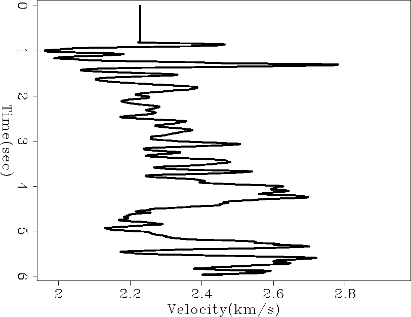 |
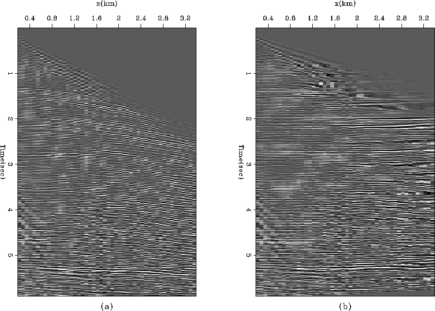
The result of applying the NMO correction with the estimated velocity function is shown in Figure 6b. Data are flattened in most areas, especially away from the beginning of the section where there is little offset information, and before the data becomes noisier at later times. Examining the strong reflector at approximately 5.2 seconds in Figure 6a, which is in the noisier part of the record and clearly non-hyperbolic, Figure 6b shows that enough velocity information is present in order to effectively flatten the event. This result is encouraging.
 |
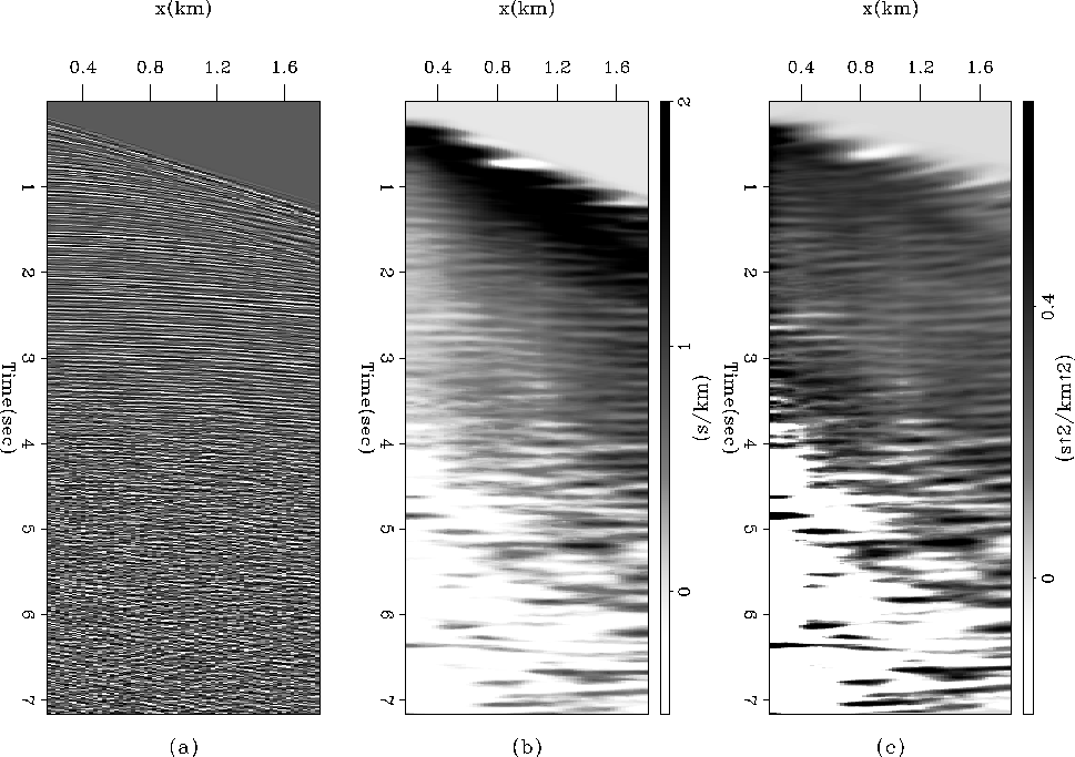
The method was also tested on shot 27 from the Yilmaz-Cumro dataset, shown in Figure 7a. The shot has numerous hyperbolas at early times, but noise levels hide hyperbolic events at later times. The dip estimate (Figure 7b) and s2 estimate (Figure 7c) each show negative values associated with the direct arrival, and the noisier part of the record but, again, these are handled by the median stacking routine.
 |
The estimated RMS velocity (Figure 8) was also extended back to zero time in order to remove bad values where there is little far offset information. The estimate seems reasonable until around 4.5s; where it starts to fluctuate. This is where the noise level in the data increases, and the poor estimate in this location occurs. The results of the NMO correction with this velocity estimate is shown in Figure 9b. Again the data has been reasonably flattened, particularly at times where the velocity estimate was well constrained.
|
27velocity
Figure 8 Estimated RMS velocity profile for the data in Figure 7. | 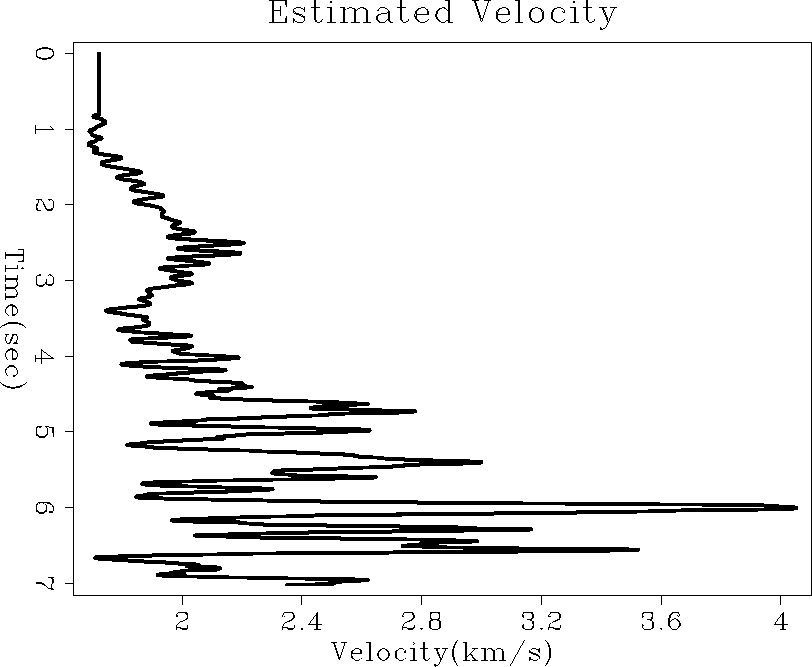 |
 |