 |
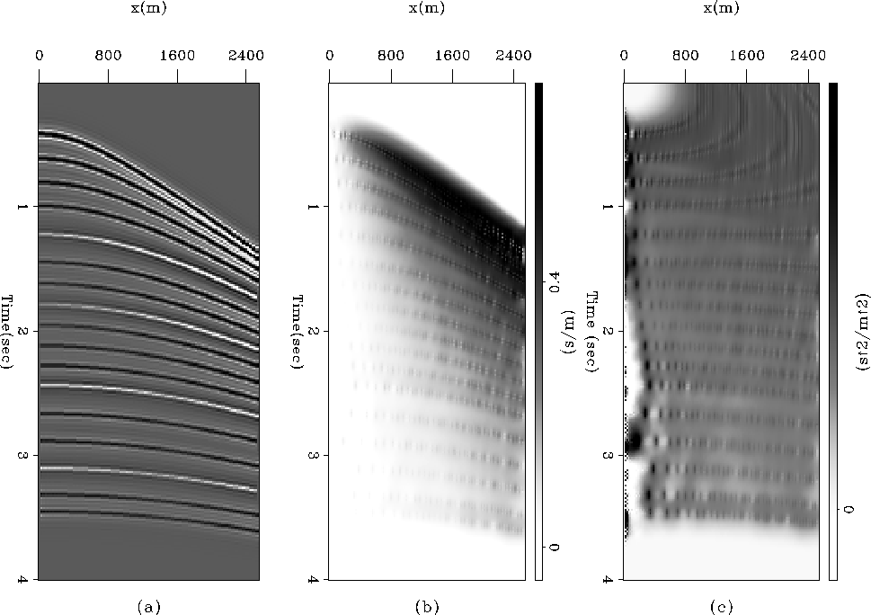
Figure 1 (a) Synthetic data, (b) estimated local dip, and (c) estimated s2 after NMO correction.
The proposed methodology was first tested on a simple synthetic example in order to check the validity of the approach. Figure 1a shows the synthetic example, which is an idealized case with neither crossing events nor aliasing, allowing robust dip estimation to occur.
 |
The variable brightness of the estimated local dip in Figure 1b represents the calculated value of dip, and shows that the estimate is robust for this simple synthetic example. Figure 1c, calculated s2 after NMO correction with the synthetic velocity profile, shows the expected trend with slowness values decreasing slightly at later times. There are some anomalous values of s2 at small offsets due to the minimal dip of the reflectors at those locations, but they will be removed by the median stacking procedure.
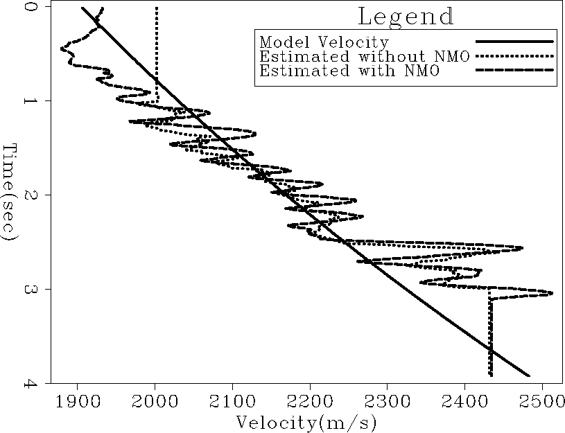
The estimated RMS velocity function of the synthetic data is shown in Figure 2. The solid line represents the velocity function used to create the synthetic data. The two dashed lines show the estimated velocity, one estimate from the orginal s2 panel, and the other from the s2 panel that has been NMO corrected (Figure 1c). The two results are similar, suggesting that in order to obtain a robust estimate of slowness the velocity used to flatten the hyperbolas of s2 before the median stack does not need to be very accurate. As long as data do not have extremely large offsets, a rough estimate of velocity for NMO correction should flatten the hyperbolas of s2 adequately, allowing the median stacking routine to obtain a reasonable estimate of s2.
|
synvelocity
Figure 2 RMS velocity profile used for the synthetic model, and estimated RMS velocity profiles with and without the NMO correction applied to the estimate of s2. |  |
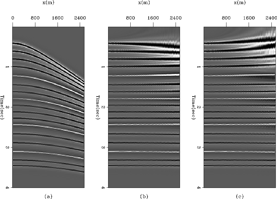
The results of using the two estimated velocity functions for NMO correction are shown in Figure 3. Figure 3b uses the s2 estimate without NMO correction, and Figure 3c uses the s2 velocity estimate with NMO correction. In both cases the estimated velocity function does a good job of flattening the hyperbolas in the synthetic data. The results are encouraging and suggest that the method will work even if the velocity for NMO correction of the plane of s2 is inaccurate.
 |