CMP gathers

 

cmp0
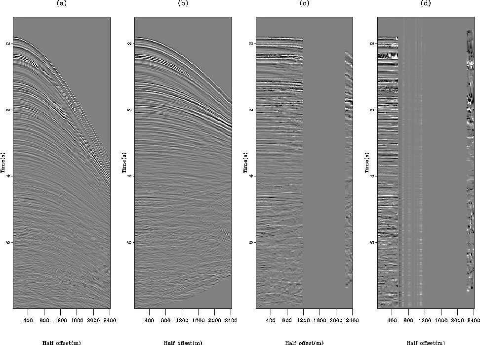
Figure 1 (a) Raw CMP gather. (b) CMP gather with constant velocity applied, 2000 $\tt ms^{-1}$. (c) Flattened version of (b) with no regularization, one iteration. (d) Flattened version of (b) with no regularization, three iterations. Notice the artifacts in (c) and (d) caused by data points being shifted without maintaining continuity and monotonicity.

Figure 1a shows a raw CMP gather. Figure 1b shows the same data after constant velocity (2000 $\tt ms^{-1}$) NMO has been applied. This reduces the maximum dip and therefore makes the dip estimation more robust. Figure 1c shows the result of one iteration of flattening with no regularization applied ($\epsilon=0$). This means that each slice of dip is integrated independently. The estimated dip can be seen in Figure 2a. Fluctuations in dip can cause horizontal striations in the time shifts as in Figure 2b. These sudden changes in time shift can cause points to be swapped in depth or time. This can create the artifacts seen in Figure 1c. These artifacts cause errors in the dip estimation which cause the problem to grow with subsequent iterations. The estimated dip for the third iteration can be seen in Figure 1c. These dips are very small compared to the dips in 1a because the figures are clipped differently. However, notice the severity of the striations in the time-shifts after the third iteration shown in Figure 2d.

 

intcmp0
Figure 2 (a) Estimated dip from (b) in Figure 1. (b) Integration result of the dip in (a). (c) Estimated dip for third iteration. (d) Integration result of the dip in (c).

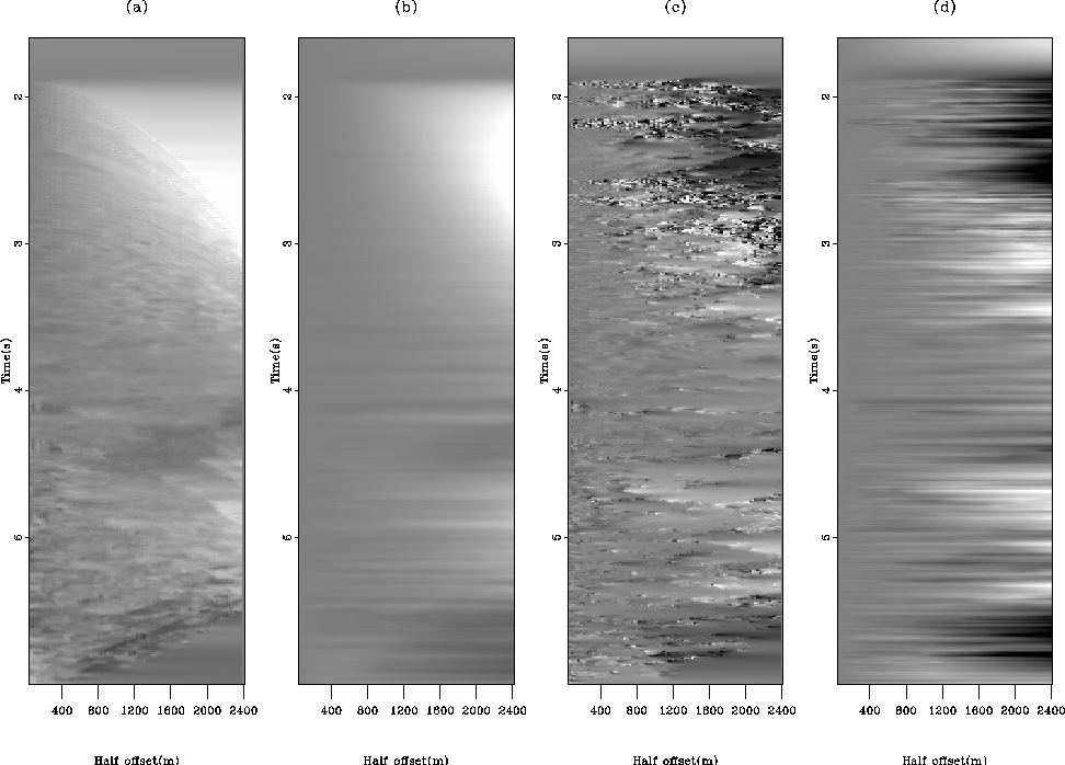
Figures 3 and 4 show the same data as Figures 1 and 2 except using regularization ($\epsilon=2$). Notice that the integrated dip shown in Figure 4b is much smoother than the result shown in Figure 2b.

After 3 iterations of flattening, Figure 3d, the gather is flat and the data is still preserved. If necessary, this data can be easily unflattened because the data integrity is intact.

 

cmp1
Figure 3 (a) Raw CMP gather. (b) CMP gather with constant velocity applied. (c) Flattened version of (b) with regularization ($\epsilon$=2), one iteration. (d) Flattened version of (b) with regularization ($\epsilon$=2), three iterations. Notice the significant improvement of the flattening result compared to Figure 1.

 

intcmp1
Figure 4 (a) Estimated dip from (b) in Figure 3. (b) Integration result of the dip in (a). (c) Estimated dip for third iteration. (d) Integration result of the dip in (c).

 

compcmpo
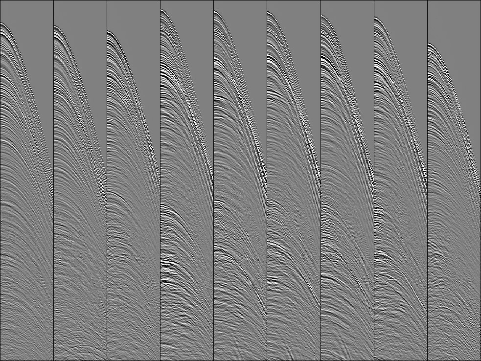
Figure 5 9 sample gathers from the same data used to create a 2D stack section. Each gather is 2600 meters apart.