Calibration

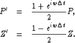
The pressure component (P) and the vertical component (Z) of the receiver gather are both in the frequency domain. The available data are the hydrophone component (P) and the non-calibrated geophone component (${\widehat Z}=\frac{Z}{C}$,C is the calibration factor we need to compute):

$$\begin{eqnarray} P & = & U+D, \nonumber \\ Z & = & \frac{U-D}{\rho v_p}. \end{eqnarray}$$ (2)

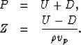
The initial source wavefield is given as follows:

 

S₀ = U₀ + D₀. (3)

The propagated upgoing and downgoing wavefields at the water-bottom surface are, respectively,

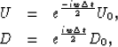$$\begin{eqnarray} U & = & e^{\frac{-iw\Delta t}{2}}U_0, \nonumber \\ D & = & e^{\frac{iw\Delta t}{2}}D_0, \end{eqnarray}$$ (4)

where $\Delta t = 2 \Delta z /v$, $\Delta z$ is the water depth and v is the water velocity. From equations (3) and (4) the propagated source at the water-bottom surface is as follows:  

$$S = D + e^{iw\Delta t}U.$$ (5)

The calibration methodology assumes that the source energy should be zero after a time equal to the sum of the source-receiver propagation time and the source duration, which is a few hundred milliseconds. Combining equations (2) and (5) yields the following relation between the propagated source (S) and the hydrophone (P) and geophone (Z) components:

S = P' - CZ', (6)

where:

$$\begin{eqnarray} P' & = & \frac{1+e^{iw\Delta t}}{2}P, \nonumber \\ Z' & = & \frac{1-e^{iw\Delta t}}{2}Z. \nonumber \end{eqnarray}$$

The propagated source vanishes after a certain period of time if the hydrophone and geophone are calibrated. This corresponds to finding C such that the propagated source (S) has minimum energy after a period of time:  

$$\min_{S} \ \ \vert\vert S_{[a,b]} \vert\vert^2.$$ (7)

The solution for this simple least-squares problem is as follows:  

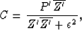$$C = \frac{P' \overline{Z'}}{Z' \overline{Z'} + \epsilon^2},$$ (8)

where $\epsilon$ is a small constant to avoid dividing by zero.

The filter C [equation (8)] is for a single trace. To obtain a filter for the entire gather, we compute the filter C for each trace and average them.

Figure 6 shows the hydrophone component of the receiver gather (left), the geophone component of the receiver gather (center) and the calibrated geophone (left).

 

cal
Figure 6 From left to right: hydrophone, geophone and calibrated geophone.