![\begin{eqnarray}
\Delta \mathcal R_b&=& \sum_\omega\left(\mathcal U- \mathcal U_...
...r} \right\vert _{\r=\r_o} \left[\mathcal R_o\right]\; \Delta \r\;.\end{eqnarray}](img42.gif)
![\begin{eqnarray}
\Delta \mathcal R_b&=& \sum_\omega\left(\mathcal U- \mathcal U_...
...r} \right\vert _{\r=\r_o} \left[\mathcal R_o\right]\; \Delta \r\;.\end{eqnarray}](img42.gif) |
(21) | |
| (22) | ||
| (23) |
Figure ![[*]](http://sepwww.stanford.edu/latex2html/cross_ref_motif.gif) shows the slowness
backprojection for image perturbations computed using the
definition in equation (21). From top to bottom,
the panels correspond to increasing magnitudes of the
slowness anomalies. In panel (a), the accumulated
differences between the background and correct images
is small, such that the Born approximation holds and
the backprojection creates simple ``fat rays''
Woodward (1992).
However, as the slowness anomaly increases,
the fat rays are distorted by sign changes (b),
and/or by the characteristic ellipsoidal side-lobes (c).
shows the slowness
backprojection for image perturbations computed using the
definition in equation (21). From top to bottom,
the panels correspond to increasing magnitudes of the
slowness anomalies. In panel (a), the accumulated
differences between the background and correct images
is small, such that the Born approximation holds and
the backprojection creates simple ``fat rays''
Woodward (1992).
However, as the slowness anomaly increases,
the fat rays are distorted by sign changes (b),
and/or by the characteristic ellipsoidal side-lobes (c).
|
RYTOV3b.xbsbor
Figure 3 Fat rays for an image perturbation defined using the Born equation (21). The slowness anomaly is gradually increasing from (a) to (c). Only the smallest anomaly is correctly handled by the Born image perturbation. | 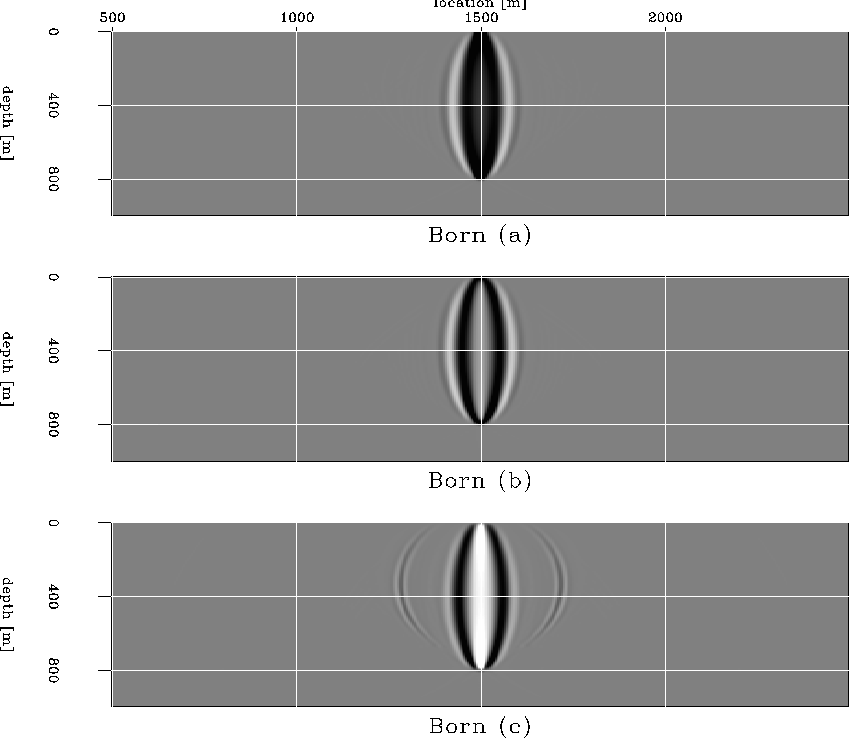 |
Figure ![[*]](http://sepwww.stanford.edu/latex2html/cross_ref_motif.gif) shows the slowness
backprojection for image perturbations computed using the
definition in equation (22). From top to bottom,
the panels correspond to increasing magnitudes of the
slowness anomalies. In panels (a) and (b), the accumulated
phase differences between the background and correct images
are small and do not wrap.
Backprojection by WEMVA also creates simple undistorted
fat rays. At large magnitudes, however, the phases become
large enough to wrap, and backprojection from image
perturbations defined by equation (22) fails (c).
shows the slowness
backprojection for image perturbations computed using the
definition in equation (22). From top to bottom,
the panels correspond to increasing magnitudes of the
slowness anomalies. In panels (a) and (b), the accumulated
phase differences between the background and correct images
are small and do not wrap.
Backprojection by WEMVA also creates simple undistorted
fat rays. At large magnitudes, however, the phases become
large enough to wrap, and backprojection from image
perturbations defined by equation (22) fails (c).
|
RYTOV3b.xbsryt
Figure 4 Fat rays for an image perturbation defined using the Rytov equation (22).The slowness anomaly is gradually increasing from (a) to (c). The phases are not unwrapped, thus the largest anomaly is not described correctly. | 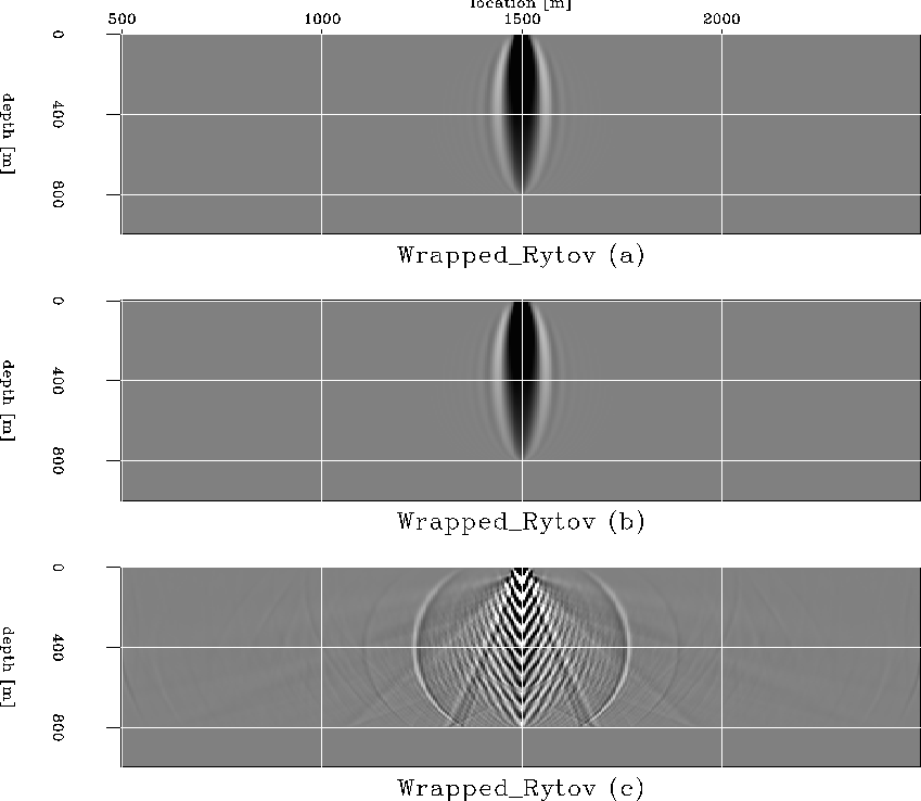 |
Both equation (21) and equation (22) employ the same operator for backprojection. The difference is in the method we use to define the wavefield perturbation. For equation (21) we use the difference between the complete wavefields, with the constraint of small total wavefield difference. For equation (22) we use the difference between the cumulative phases, which does not impose a constraint on the actual size of the wavefields. Thus, using equation (22), we could in principle handle arbitrarily large slowness perturbations.
However, the phases in equation (22) need to be
unwrapped to obtain a meaningful wavefield differences.
In complex environments, wavefields are can be quite
complicated, and it is not at all
trivial to estimate and unwrap their phases.
Therefore, even if we could in theory
use equation (22) for arbitrarily large perturbations,
in practice we are constrained by our ability to
unwrap the phases of complicated wavefields.
Figure ![[*]](http://sepwww.stanford.edu/latex2html/cross_ref_motif.gif) shows the fat rays
corresponding to the different magnitudes of slowness
anomalies when the phases have been unwrapped.
shows the fat rays
corresponding to the different magnitudes of slowness
anomalies when the phases have been unwrapped.
|
RYTOV3b.xbsunw
Figure 5 Fat rays for an image perturbation defined using the Rytov equation (22).The slowness anomaly is gradually increasing from (a) to (c). The phases are unwrapped, thus all anomalies are described correctly. | 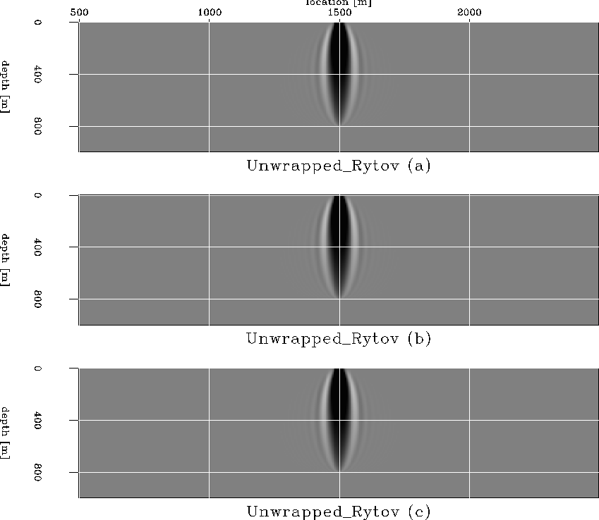 |
The more practical alternative we can use to create
image perturbations using equation (23)
is illustrated in Figure ![[*]](http://sepwww.stanford.edu/latex2html/cross_ref_motif.gif) .
In this case, the fat rays are not distorted at any
magnitude of slowness anomaly, behavior which is
similar to that of the unwrapped Rytov.
.
In this case, the fat rays are not distorted at any
magnitude of slowness anomaly, behavior which is
similar to that of the unwrapped Rytov.
|
RYTOV3b.xbsana
Figure 6 Fat rays for an image perturbation defined using the differential equation (23).The slowness anomaly is gradually increasing from (a) to (c). All anomalies are described correctly. | 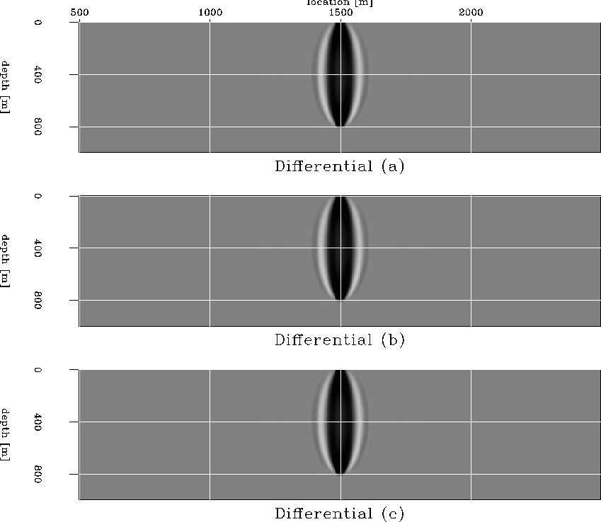 |
The explanation for this behavior lies in the definition
in equation (23). The image perturbation is
created by estimating the gradient of the residual migration
change on the background image, followed by scaling with
the appropriate ![]() picked from a suite of images
obtained with different values of the parameter
picked from a suite of images
obtained with different values of the parameter ![]() .
.
In essence, we are using the information provided by the
background image to infer the direction and magnitude of
the image change. There is no limitation to how far we can go
from the background image similar to the limitations of
the Born and Rytov definitions. However, since we are
employing a first order linearization, the accuracy of the
differential image perturbation decreases with increasing
![]() .
.
|
dif
Figure 7 A sketch of the approximations done when computing image perturbations with equation (23). In this plot, each multi-dimensional image is schematically depicted by a point. We compute a linear approximation of an image corresponding to a spatially varying | 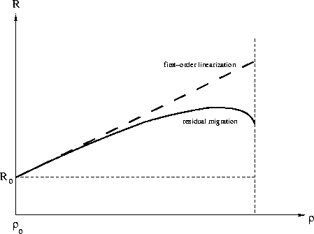 |
Figure ![[*]](http://sepwww.stanford.edu/latex2html/cross_ref_motif.gif) is a schematic illustration
of the transformation implied by equation (23).
We can create enhanced images either by nonlinear residual
migration, or by a first-order linearization around the
background image. In principle, the accuracy of this
approximation decreases with increasing
is a schematic illustration
of the transformation implied by equation (23).
We can create enhanced images either by nonlinear residual
migration, or by a first-order linearization around the
background image. In principle, the accuracy of this
approximation decreases with increasing ![]() . Therefore,
in practice we cannot go arbitrarily far from any given
background image and we need to run several non-linear
iterations involving slowness inversion, re-migration and
re-linearization.
. Therefore,
in practice we cannot go arbitrarily far from any given
background image and we need to run several non-linear
iterations involving slowness inversion, re-migration and
re-linearization.
Figure ![[*]](http://sepwww.stanford.edu/latex2html/cross_ref_motif.gif) is a summary of fat rays computed
using the methods described in the preceding section.
The magnitude of the slowness anomaly increases from left
to right. From bottom to top we show the fat rays for
the Born definition,
the Rytov definition without phase unwrapping,
the Rytov definition with phase unwrapping, and
the differential definition.
is a summary of fat rays computed
using the methods described in the preceding section.
The magnitude of the slowness anomaly increases from left
to right. From bottom to top we show the fat rays for
the Born definition,
the Rytov definition without phase unwrapping,
the Rytov definition with phase unwrapping, and
the differential definition.
The four panels on the left are identical, since all methods work as well for small anomalies. In the middle four panels, the fat ray obtained with the Born definition starts to break, while the Rytov (with and without phase unwrapping) and differential approaches work well. Finally, the panels on the right correspond to the highest anomaly, when only the Rytov with phase unwrapping and differential methods work.