SINGULAR VALUE DECOMPOSITION

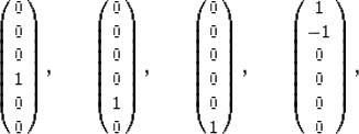
The singular value decomposition (SVD), or equivalently the eigenvalue decomposition in the case of a real symmetric matrix, for (1) is relatively easy to perform. We can immediately write down four eigenvectors:

$$\begin{eqnarray} \left( \begin{array} {c} 0 \ 0 \ 0 \ 1 \ 0 \ 0 \ \en... ...ray} {c} 1 \ -1 \ 0 \ 0 \ 0 \ 0 \ \end{array}\right), \end{eqnarray}$$ (26)

and their corresponding eigenvalues, respectively 2l, 2l, 2m, and a-b = 2m. All four correspond to shear modes of the system. The two remaining eigenvectors must be orthogonal to all four of these and therefore both must have the general form

$$\begin{eqnarray} \left( \begin{array} {c} 1 \ 1 \ X\ 0 \ 0 \ 0 \ \end{array}\right), \end{eqnarray}$$ (27)

with the corresponding eigenvalue

$$\begin{eqnarray} \chi = a + b + f X. \end{eqnarray}$$ (28)

The remaining condition that determines both X and $\chi$is

$$\begin{eqnarray} \chi X= 2f + c X, \end{eqnarray}$$ (29)

which, after substitution for $\chi$, leads to a quadratic equation having the solutions

$$\begin{eqnarray} X_{\pm} = {{1}\over{2}}\left(-\left[{{a + b - c}\over{f}}\right] \pm\sqrt{8 + \left[{{a + b - c}\over{f}}\right]^2}\right). \end{eqnarray}$$ (30)

The ranges of values for $X_\pm$ are $0 \le X_+ \le \infty$ and, since X_- = -2/X₊, $-\infty \le X_- \le 0$.The interpretation of the solutions $X_\pm$ is simple for the isotropic limit where X₊ = 1 and X_- = -2, corresponding respectively to pure compression and pure shear modes. For all other cases, these two modes have mixed character, indicating that pure compression cannot be excited in the system, and must always be coupled to shear. 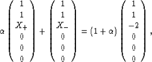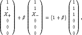Some types of pure shear modes can still be excited even in the nonisotropic cases, because the other four eigenvectors in (26) are unaffected by this coupling, and they are all pure shear modes. Pure compressional and shear modes are obtained as linear combinations of these two mixed modes according to

$$\begin{eqnarray} \alpha \left( \begin{array} {c} 1 \ 1 \ X_+ \ 0 \ 0 \ ... ...ray} {c} 1 \ 1 \ -2 \ 0 \ 0 \ 0 \ \end{array}\right), \end{eqnarray}$$ (31)

with $\alpha = -2(X_+-1)/[X_+(X_+ + 2)]$for pure shear, and

$$\begin{eqnarray} \left( \begin{array} {c} 1 \ 1 \ X_+ \ 0 \ 0 \ 0 \ \... ...rray} {c} 1 \ 1 \ 1 \ 0 \ 0 \ 0 \ \end{array}\right), \end{eqnarray}$$ (32)

and with $\beta = X_+(X_+ - 1)/(X_+ + 2)$for pure compression.

To understand the behavior of X₊ in terms of the layer property fluctuations or, alternatively, in terms of the Thomsen parameters, it is first helpful to note that the pertinent functional $F(x) = {{1}\over{2}}\left[-x + \sqrt{8 + x^2}\right]$ is easily shown to be a monotonic function of its argument x. So it is sufficient to study the behavior of the argument x = (a+b-c)/f.

 

• Exact results in terms of layer elasticity parameters
• Approximate results for small values of Thomsen parameters