Gradient magnitude and Laplacian regularization

In the previous section we changed the norm of the minimization problem to prevent the roughener from smoothing over the edges of the model. In this subsection we shift from a statistical to a more mechanical approach to attain the same goal.

The gradient magnitude ($\vert\vert\nabla\vert\vert$) is an isotropic edge-detection operator that can be used to calculate the diagonal weights. Unfortunately, it is a nonlinear operator thus couldn't be used for regularization. Instead we used the Laplacian, which is a regularization operator used in several SEP applications Claerbout and Fomel (2001).

The gradient magnitude edge-preserving regularization fitting goal was set following the nonlinear iterations: starting with ${\bf Q_{\vert\vert\nabla\vert\vert}}^{0} = \bf I$, at the k^th iteration the algorithm solves

$$\begin{eqnarray} {\bf Kf}^{k} - { \bf g \approx 0 } \nonumber \\ {\bf \epsilon ... ...vert\nabla\vert\vert}}^{k-1} { \bf \nabla^2 f}^k { \bf \approx 0 }\end{eqnarray}$$ (3)

where  

$${\bf Q_{\vert\vert\nabla\vert\vert}}^{k-1} = \frac{1}{1+ \frac{{ \bf \vert\vert\nabla f}^{k-1}\vert\vert}{\alpha} }.$$ (4)

$\bf K$ is a non-stationary convolution matrix, ${\bf f}^{k}$ is the result of the k^th nonlinear iteration, ${\bf Q_{\vert\vert\nabla\vert\vert}}^{k-1}$ is the (k-1)^th diagonal weighting operators, $\bf I$ is the identity matrix, ${ \bf \vert\vert\nabla\vert\vert}$ is the gradient magnitude, ${ \bf \nabla^2}$ is the Laplacian operator, the scalar $\alpha$ is the trade-off parameter controlling the discontinuities in the solution, and the scalar $\epsilon$ balances the relative importance of the data and model residuals.

 

comp_images_laplac_2d
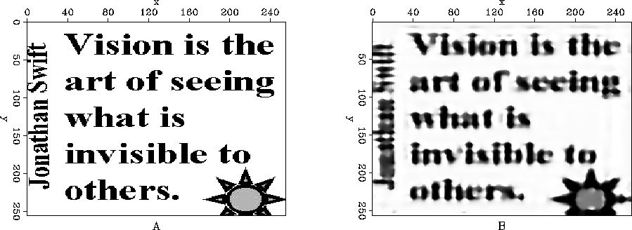
Figure 6 A) Original image, B) Deblurred image using LS with the gradient magnitude edge-preserving regularization ($\vert\vert\nabla\vert\vert$) with laplacian edge-preserving regularization

 

comp_graph_2d_laplac
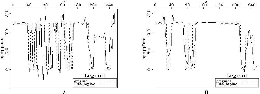
Figure 7 Comparison between Figures A and B; A) Slice y=229 and B) Slice x=229.

Figures  and show a considerable improvement over Figures  and . They are noise free but keep the round features of the original image. However, since we are not imposing blockiness on the model but rather on the derivative of the model (using the Laplacian as the regularization operator), the edges are not as sharp as the previous case.