Tomography Review

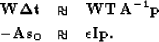
Following the methodology of Clapp and Biondi (1999), I will begin by considering a regularized tomography problem. I will linearize around an initial slowness estimate and find a linear operator in the vertical traveltime domain $\bf T_{}$ between our change in slowness $\bf \Delta s$and our change in traveltimes $\bf \Delta t$.We will write a set of fitting goals,

$$\begin{eqnarray} \bf \Delta t&\approx&\bf T_{} \bf \Delta s\nonumber \\ \bf 0&\approx&\epsilon \bf A\bf \Delta s,\end{eqnarray}$$ (1)

where $\bf A$ is our steering filter operator Clapp et al. (1997) and $\epsilon$ is a Lagrange multiplier. However, these fitting goals don't accurately describe what we really want. Our steering filters are based on our desired slowness rather than change of slowness. With this fact in mind, we can rewrite our second fitting goal as:

$$\begin{eqnarray} \bf 0&\approx&\epsilon \bf A\left( {\bf s_0} + \bf \Delta s\rig... ...mber -\epsilon \bf A{\bf s_0} &\approx&\epsilon \bf A\bf \Delta s.\end{eqnarray}$$ (2)

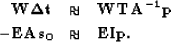
Our second fitting goal can not be strictly defined as regularization but we can still do a preconditioning substitution Fomel et al. (1997), giving us a new set of fitting goals:

$$\begin{eqnarray} \bf \Delta t&\approx&\bf T_{} \bf A^{-1}\bf p\nonumber \\ - \epsilon \bf A{\bf s_0} &\approx&\epsilon \bf I\bf p .\end{eqnarray}$$ (3)

Our standard inversion fitting goals (3) make an assumption that our data fitting goal is equally believable everywhere. Stated another way, we want the same weight $\epsilon$ for our model styling goal everywhere. This is generally untrue. We can, and should, account for differing level of confidence in two different ways. If we have a measure of certainty about a data point (for example how much of a peak our semblance pick is) we can add a data covariance operator $\bf W$ to our fitting goals,

$$\begin{eqnarray} \bf W \bf \Delta t&\approx&\bf W \bf T_{} \bf A^{-1}\bf p \nonumber \\ - \bf A{\bf s_0} &\approx&\epsilon \bf I\bf p.\end{eqnarray}$$ (4)

We can also often make statements about our confidence in our data fitting goal as a function of our model space. For example, generally as we get deeper, we will have less confidence in the points, and be less able to get a high frequency velocity model. We can account for this uncertainty by replacing the constant epsilon of fitting goal (4) with a diagonal weighting operator $\bf E$ resulting in the updated fitting goals,

$$\begin{eqnarray} \bf W \bf \Delta t&\approx&\bf W \bf T_{} \bf A^{-1}\bf p\nonumber \\ - \bf E \bf A{\bf s_0} &\approx&\bf E \bf I\bf p .\end{eqnarray}$$ (5)

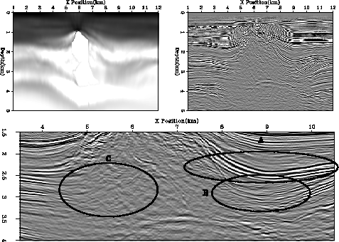
By having this additional freedom we can allow for more model variability in the near surface and force more smoothing at deeper locations. Figure 6 shows the result of using the new fitting goals (5). Note how we have a higher frequency velocity structure above and a smoother below. The overall image quality is also improved compared to Figure 5.

 

combo.vel1.eps
Figure 6 Data after one iteration using a constant $\epsilon$. The top-left panel shows the velocity model and the top-right panel shows the migrated image using this velocity. The bottom panel shows a zoomed area around the salt body. Note the salt bottom,`A'; the valley structure at `B'; and under the salt over-hang at `C'. Note the improved image quality compared to Figure 4 and Figure 5.