L₁ norm to handle large residuals

The previous section discussed a method to reduce the number of bad data points. Another approach is to limit their effect in the inversion. Generally we do not iterate to convergence. Early iterations tend to concentrate on large residuals. Erroneous data points tend to cause the large residuals. The result is that our solutions tend to be dominated by these erroneous data points.

A method to combat this problem is to change our misfit functional from the traditional

$$\bf r_d = \Vert \bf d - \bf L \bf m\Vert^2 .$$ (6)

There are two different methods to change the misfit function. The first is to use a non-linear solver. With a non-linear solver there are a variety of misfit functions, most interestingly the $\L _1$ and Huber functionals Claerbout (1996); Clapp and Brown (1999); Huber (1973). A second approach is reweighted least-squares, Guitton (2000); Nichols (1994). In reweighted least-squares a weighting operator is applied to the residuals based upon the size of residuals at certain points in the inversion.

The total non-linear approach has fewer parameters to manipulate and is generally more robust than reweighted approach. The downside of the completely non-linear approach is that it is significantly slower (a factor of ten or more is not uncommon). I chose the reweighted least-squares approach because I am most interested in finding and minimizing the effect of the largest residuals. I found that a single calculation of the weighting function after $\frac{1}{3}$ of the total number of iterations was sufficient to minimize the most troublesome residuals. 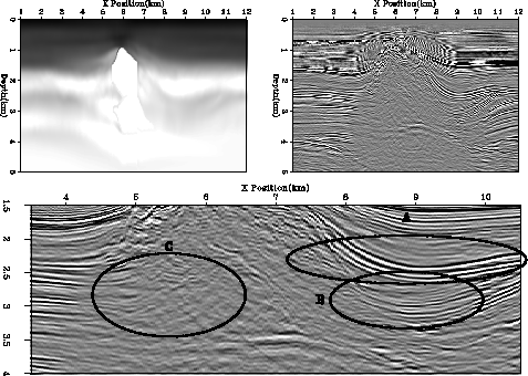Figure 7 shows the velocity and migration result using an L₁ norm. Note the improvement in image quality over either of the previous approaches (Figures  4 and 5). The salt bottom is more continuous, `A'. The valley structure is better defined, `B'. The reflectors are more continuous and extend closer to the salt at `C'.

 

combo.vel1.steer
Figure 7 Data after one non-linear iteration using a reweighted least-squares. The top-left panel shows the velocity model and the top-right panel shows the migrated image using this velocity. The bottom panel shows a zoomed area around the salt body. Note the salt bottom,`A'; the valley structure at `B'; and under the salt over-hang at `C'. Note the improved image quality compared to Figure 4 and Figure 5.