Test with synthetic data (convolutional model)

We tested the different implementations of the imaging condition with synthetic data. The data simulates the case when source and receiver wavefields coincide at reflector depth and the case when they coincide at a shallower depth. The data are constructed by convolving a minimum-phase, 25 Hz central frequency, band-limited wavelet with a series of spikes.

Figure  shows the deconvolution of the signal by itself. The signal was constructed by convolving the wavelet with two spikes. This simulates the situation where source and receiver wavefields coincide at reflector depth. As expected, the result is a delta function centered at zero lag with no difference between the two deconvolution methods (Figures d and e). Figure c shows the result of the cross-correlation for the sake of comparison. The cross-correlation result differs from the deconvolution result in resolution, but still is a symmetric function centered at zero lag.

 

shift
Figure 4 Source and receiver wavefields shifted from zero, simulating wavefields coinciding at the reflector depth. (a) Source wavefield (b) Receiver wavefield (c) Cross-correlation (d) Deconvolution (b) by (a) in the time domain (e) Deconvolution (b) by (a) in the Fourier domain.

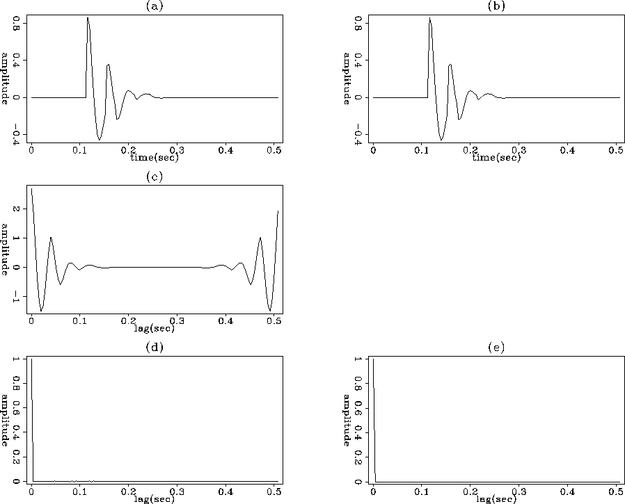Figure  shows the result of deconvolving the same signal shifted to the right (Figure b) by the unshifted signal (Figure a). This simulates the situation where the receiver and the source wavefield coincide at a depth shallower than the reflector depth. The result is a shifted delta function. No significant differences can be seen between the two convolution methods. In this situation the cross-correlation (Figure c) produces an erroneous image since the zero lag is different than zero.

 

shift_dt
Figure 5 Source and receiver wavefields shifted from zero and each others, simulating wavefields coinciding at a depth shallower the reflector depth. (a) Source wavefield (b) Receiver wavefield (c) Cross-correlation (d) Deconvolution (b) by (a) in the time domain (e) Deconvolution (b) by (a) in the Fourier domain.

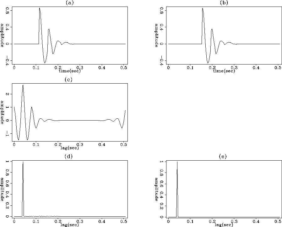Figure  shows the deconvolution of the same signal (in Figure b) contaminated by more spikes (Figure b) with the original signal (Figure a). This resembles a real situation when source and receiver wavefields coincide at reflector depth. The deconvolution method based on least squares inversion in time gets the correct value at zero lag but does not converge to the global minimum. In the Fourier domain the delta at zero is recuperated and some energy comes at the end of the signal due to symmetric boundary conditions. Since we are only interested in the zero lag value, both deconvolution methods could be used. The result of the cross-correlation (Figure c) has a maximum at zero lag as expected.

 

shift_mult
Figure 6 Source and receiver wavefields shifted from zero. It simulates two wavefields coinciding at the reflector depth. Receiver wavefield contaminated with more events. (a) Source wavefield (b) Receiver wavefield (c) Cross-correlation (d) Deconvolution (b) by (a) in the time domain (e) Deconvolution (b) by (a) in the Fourier domain.

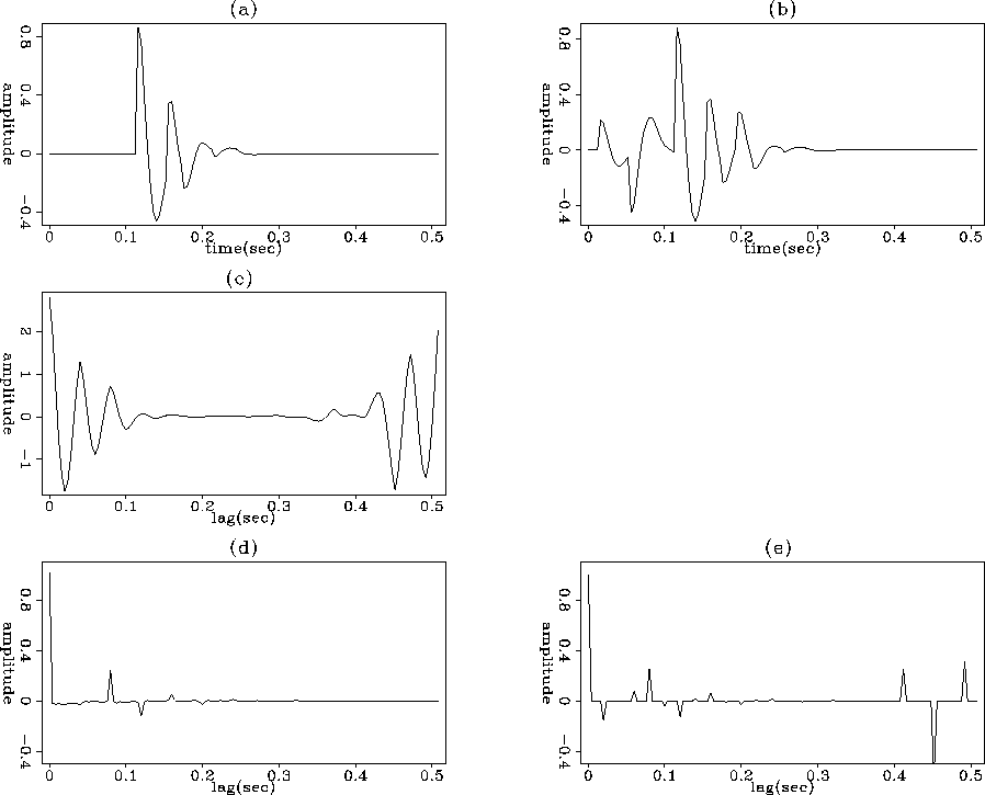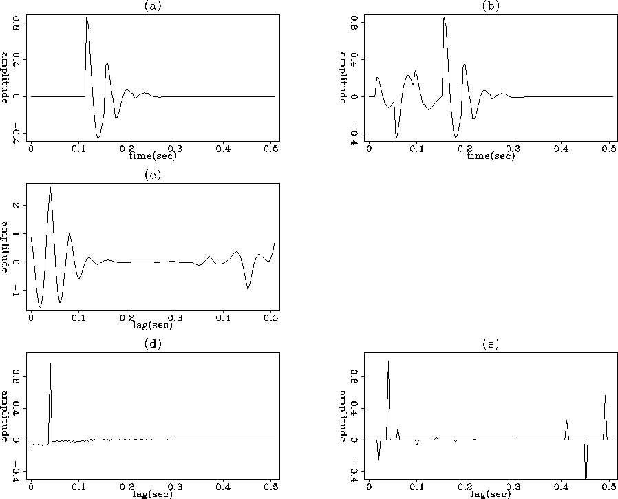
Figure  shows the deconvolution of the same signal (in Figure b) shifted to the right (Figure b). This simulates the situation where the receiver and the source wavefield coincide at a depth shallower than the reflector depth. The deconvolution method based on least squares inversion in the time domain recovers the correct shifted spike. As we saw in the previous case, when some energy exist before the onset of the reflector energy in the receiver wavefield, the least squares fails to reach the global minimum. In the Fourier domain, we recover the shifted spike and some energy comes at the end of the signal due to symmetric boundary conditions. In this case the deconvolution in the Fourier domain has a better performance than the deconvolution in the time domain since there is no energy at zero lag, as was theoretically predicted.

 

shift_mult_dt
Figure 7 Source and receiver wavefields shifted from zero and each others. It simulates two wavefields coinciding at a depth shallower the reflector depth. Receiver wavefield contaminated with more events. (a) Source wavefield (b) Receiver wavefield (c) Cross-correlation (d) Deconvolution (b) by (a) in the time domain (e) Deconvolution (b) by (a) in the Fourier domain.