


Next: Deconvolution in the Fourier
Up: Valenciano and Biondi: Deconvolution
Previous: Reflector mapping imaging condition
Deconvolution in the time domain can be implemented in terms of the following fitting goal for each (x,z) location:
|  |
(4) |
where  is a convolution matrix whose columns are downshifted versions of the source wavefield
  .
.
The least-squares solution of this problem is
where  is the adjoint of .A damped solution may be used to guarantee
  to be invertible as in
where
to be invertible as in
where  is a small positive number.
Equation (6) can be written in terms of the fitting goals
is a small positive number.
Equation (6) can be written in terms of the fitting goals
| 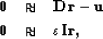 |
(5) |
| |
where  is the identity matrix.
This approach can be computational efficient if the time window is not too large and we use a Conjugate Gradient as optimization engine. However, it has the disadvantage of relying on a linear inversion process that may or may not converge to the global minimum.
A way to overcome this problem, obtaining an analytical solution, is to implement equation (6) in the Fourier domain, as we do in the next section.
is the identity matrix.
This approach can be computational efficient if the time window is not too large and we use a Conjugate Gradient as optimization engine. However, it has the disadvantage of relying on a linear inversion process that may or may not converge to the global minimum.
A way to overcome this problem, obtaining an analytical solution, is to implement equation (6) in the Fourier domain, as we do in the next section.
Next: Deconvolution in the Fourier
Up: Valenciano and Biondi: Deconvolution
Previous: Reflector mapping imaging condition
Stanford Exploration Project
11/11/2002