


Let us consider the explicit finite-difference scheme for the full wave equation
| (8) |
| |
(9) |
![]()
![]()
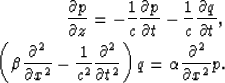
Let us consider the wavefield on the boundary z=Zmax. There are only outgoing waves at z=Zmax, so the wavefield satisfies the downgoing wave equation, for which we can write its approximate equations:
 |
(10) | |
| (11) |
For compatibility with the explicit finite-difference scheme at internal points, we apply the explicit finite-difference scheme for the boundaries using equation (10) and (11) and get
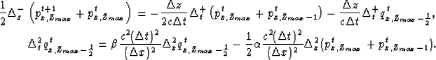 |
(12) | |
| (13) |
![]()
![]()
Assuming that the wavefield px,zk for ![]() is known,
then we solve the internal equation
(9) to get the wavefield for the internal points
Xmin<x<Xmax, Zmin<z<Zmax at time t+1, px,zt+1
first. Then, the auxiliary wavefield
is known,
then we solve the internal equation
(9) to get the wavefield for the internal points
Xmin<x<Xmax, Zmin<z<Zmax at time t+1, px,zt+1
first. Then, the auxiliary wavefield ![]() can be solved by equation (13) since the wavefield of the boundary
at time t, ptx,Z<<275>>max and ptx,Z<<276>>max-1
are known. Finally, we solve equation (12) to get the wavefield
at the boundary ptx,z=Z<<278>>max. Figure 1 illustrates how the boundary conditions are solved.
can be solved by equation (13) since the wavefield of the boundary
at time t, ptx,Z<<275>>max and ptx,Z<<276>>max-1
are known. Finally, we solve equation (12) to get the wavefield
at the boundary ptx,z=Z<<278>>max. Figure 1 illustrates how the boundary conditions are solved.
|
boundary
Figure 1 solution at the boundary z=Zmax | 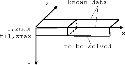 |

The method of solving the wavefield at the other three boundaries z=Zmin, x=Xmin, and x=Xmax, is similar to that of boundary z=Zmax. The only difference is that the boundary condition equation is an upgoing wave equation at z=Zmin, leftgoing wave equation at x=Xmin, and right-going wave equation at x=Xmax.
According to Zhang and Wei (1998), this absorbing boundary condition is stable.