Estimation of systematic error from crossing points

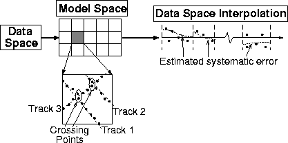
It is fairly easy to compute ``crossing points'' from the raw data. I partition the data spatially into fairly small regions and, using a Fortran90 data structure, store the track index of each data point in the region. I decide that two data points cross if they belong to different tracks and are separated (spatially) by a distance less than a predefined threshold.

Unraveling the distribution of errors between the two crossing points is a much more difficult, and possibly intractable problem, in the absence of prior information. In general, each of the two crossing points contain an unknown combination of systematic and random error. In this case, I simply ``split the difference'' by assuming that, given a measured difference between two crossing points, the systematic error is distributed evenly between the two points.

Once I have a series of measured differences at crossing points, I estimate the systematic error at all points in the data space by solving a least squares missing data problem. I impose the assumption that the systematic error is smooth along acquisition tracks by adding a roughness penalty to the least squares objective function. In least squares fitting goals, these ideas are written as follows.

$$\begin{eqnarray} \bf W_e(Ke - Ke_d) &\approx& \bf 0 \nonumber \\ \bf \nabla e &\approx& \bf 0\end{eqnarray}$$ (4)

$\bf e_d$ is the measured differences at crossing points. e is the estimated systematic error. The reliability of the measured difference is inversely proportional to the spatial separation distance of the two crossing points, r. Arbitrarily, I choose the residual weight, $\bf W_e$, for a pair of crossing points as (1 - (r/r₀)²), where r₀ is the predefined threshold which defines crossing points. K is a selector matrix. Figure 1 outlines the scheme.

 

crosspoint
Figure 1 Algorithm for estimating systematic data error by inverting crossing point data. Data is partitioned into local regions, where crossing point differences are computed. The optimization of equation (4) operates in the data space. The measured crossing point differerences are the data; we use least squares to fit a smooth trend to the measured data. The optimization operates independently on individual tracks.