


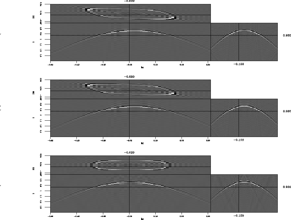
Figure 1 shows the impulse response of the three residual prestack migration operators [equations (3), (5), (6)].
 |
![[*]](http://sepwww.stanford.edu/latex2html/movie.gif)


Figure 1a presents the impulse
response for equation (3), with
![]() ,
, ![]() and
and ![]() .Figure 1b presents
the impulse response for equation (5),
with
.Figure 1b presents
the impulse response for equation (5),
with ![]() and
and ![]() .As expected
from the theory discussed in the previous section,
Figure 1a and
Figure 1b are identical
because
.As expected
from the theory discussed in the previous section,
Figure 1a and
Figure 1b are identical
because ![]() .
.
Figure 1c presents the impulse response
for equation (6), with
![]() ,
, ![]() . It is possible to
observe the difference with respect to figures
1a and 1b. The difference
is due to the approximation in the transformation
kernel.
. It is possible to
observe the difference with respect to figures
1a and 1b. The difference
is due to the approximation in the transformation
kernel.
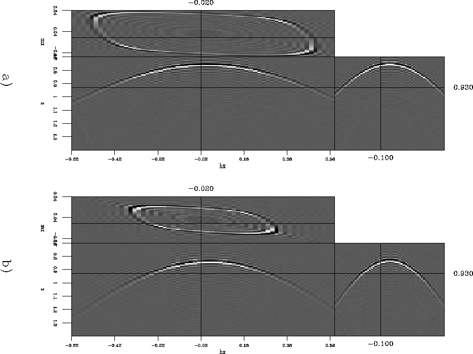
Figure 2 demonstrates
the differences between
equations (3) and (5).
Figure 2a
shows the impulse response for equation (3)
with,
![]() ,
, ![]() and
and ![]() .Figure 2b
shows the impulse response for equation (5)
with,
.Figure 2b
shows the impulse response for equation (5)
with,
![]() and
and ![]() .It is easy to observe the difference between the
impulse responses due to the approximation in
the transformation kernel.
.It is easy to observe the difference between the
impulse responses due to the approximation in
the transformation kernel.
 |