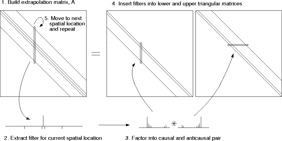
![[*]](http://sepwww.stanford.edu/latex2html/cross_ref_motif.gif) illustrates a process for factorizing a
non-stationary filtering matrix.
This approach is accurate if the filters vary smoothly in space, and
it is the approach that I follow for the examples in this chapter.
illustrates a process for factorizing a
non-stationary filtering matrix.
This approach is accurate if the filters vary smoothly in space, and
it is the approach that I follow for the examples in this chapter.
![[*]](http://sepwww.stanford.edu/latex2html/cross_ref_motif.gif) ), we must factor
the filter into causal and anticausal components.
), we must factor
the filter into causal and anticausal components.
Figure ![[*]](http://sepwww.stanford.edu/latex2html/cross_ref_motif.gif) illustrates a process for factorizing a
non-stationary filtering matrix.
This approach is accurate if the filters vary smoothly in space, and
it is the approach that I follow for the examples in this chapter.
illustrates a process for factorizing a
non-stationary filtering matrix.
This approach is accurate if the filters vary smoothly in space, and
it is the approach that I follow for the examples in this chapter.
The first step is to build the extrapolation matrix. Then we can extract the impulse response associated with each spatial location, and factor it into causal and anticausal components. By inserting the causal components into the column of a lower triangular matrix, and the anticausal components into a row of an upper triangular matrix, we can begin to build the two invertible matrices. The process has to be repeated for each spatial location.
 |
In practice, we can save time by factoring the filters in advance,
and storing them in a table.
For every value of ![]() , we precompute the factors
of the 1-D helical filter,
, we precompute the factors
of the 1-D helical filter, ![]() , and store filter
coefficients in a look-up table.
We then extrapolate the wavefield by non-stationary convolution
[equation (
, and store filter
coefficients in a look-up table.
We then extrapolate the wavefield by non-stationary convolution
[equation (![[*]](http://sepwww.stanford.edu/latex2html/cross_ref_motif.gif) )],
followed by non-stationary polynomial division with
equation (
)],
followed by non-stationary polynomial division with
equation (![[*]](http://sepwww.stanford.edu/latex2html/cross_ref_motif.gif) ).
).
Since we interpolate filters, not downward continued wavefields as in phase-shift plus interpolation migration Gazdag and Sguazzero (1984), the number of reference velocities used has minimal effect on the overall cost of the migration. Indeed, the cost of this process is proportional to the number of grid nodes times the number of filter coefficients; so for a fixed number of filter coefficients, the cost is linear in the number of grid nodes [O(N)].