Next: Sources of inaccuracy
Up: Sava and Biondi: Amplitude-preserved
Previous: Pseudo-unitary modeling/migration
Angle-domain common-image gathers are the instrument we use to analyze
the amplitude variation with reflection angle.
As we discussed in in an earlier section,
ADCIGs can be conveniently formed in the frequency domain.
local
Figure 2 A scheme of reflection rays in an
arbitrary-velocity medium.
|
|  |

Following the derivation of Fomel (1996),
if we consider that, in constant velocity media,
t is the traveltime from the source to the reflector and back
to the receiver at the surface,
2 h is the offset between the source and the receiver,
z is the depth of the reflection point,
 is the geologic dip,
 is the reflection angle, and
s is the slowness (Figure 1),
we can write
is the reflection angle, and
s is the slowness (Figure 1),
we can write
|  |
(17) |
| (18) |
Combining Equations (17) and (18), we find that
|  |
(19) |
Equation (19) is derived in constant velocity media, but it
remains perfectly valid in a differential sense in any arbitrary
velocity media if we consider h to be the effective offset at the reflector
depth and not the surface offset (Figure 1).
In the frequency-wavenumber domain Sava and Fomel (2000),
formula (19) takes the trivial form
|  |
(20) |
This equation indicates that angle-gathers can be conveniently
formed with the help of frequency-domain migration algorithms
Stolt (1978). Furthermore, wave-equation migration is
ideally suited to compute angle-gathers using such a method,
since the migration output is precisely described by the offset at
the reflector depth, which is a model parameter, and not by the surface
offset, which is a data parameter Biondi (1999).
We can also recognize that Equation (17) describes nothing
but the ray parameter of the propagating wave at the incidence with the
reflector. Using the definition

it follows that we can write a relation similar to Equation (20)
to evaluate the offset ray parameter in the Fourier-domain:
|  |
(21) |
Both Equations (20) and (21) can be used to compute
image gathers through radial trace transforms (RTT) in the Fourier domain. The
major difference is that Equation (20) operates in the space
of the migrated image, while Equation (21) operates in the data
space.
The two methods are also different in three other ways:
- 1.
- The image-space method (20)
is completely decoupled from migration,
therefore conversion to reflection angle can be thought of as a
post-processing after migration.
Such post-processing is interesting because it allows conversion from the
angle domain back to the offset domain without re-migration
(Figure 2), which is, of course, not true for the
data-space method (21), where the transformation is a
function of the data frequency (
 ).
polarity
).
polarity
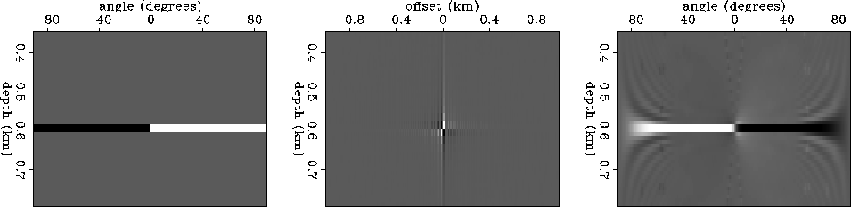
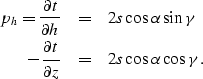
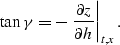
Figure 1 Synthetic example of conversion between
the angle and offset domains in the image space.
Left panel: synthetic angle gather.
Middle panel: conversion from angle to offset.
Right panel: conversion back to the angle domain.
- 2.
- From Equation (17), it follows that offset ray parameter
(ph) is also a function of the structural dip (),
which is not true for the reflection angle () estimated in the image
space. The angles we obtain using Equation (20) are geometrical
measures, completely independent on the
structural dip. For AVA purposes, it is also very convenient to have the
amplitudes as a function of reflection angle and not offset or offset
ray-parameter.
- 3.
- Both methods require accurate knowledge of the imaging velocity.
The difference is that the data-space method is less sensitive to
the location of velocity boundaries. However, conversion from ph
to reflection angle is also critically influenced by errors
in the velocity maps.
Next: Sources of inaccuracy
Up: Sava and Biondi: Amplitude-preserved
Previous: Pseudo-unitary modeling/migration
Stanford Exploration Project
4/16/2001