Pseudo-unitary modeling/migration

The ``true-amplitude'' migration defined in Equation (12) is a good approximation in the case of mild velocity variations, commonly labeled as ``time-migration'' problems. In complex overburden, the so called ``depth-migration'' situations, the reflectors are sparsely and unevenly illuminated Rickett (2001), therefore the amplitude corrections described in the preceding sections may become a poor approximation. In these cases, the amplitude term ($\bold \AA$) is neither diagonal nor invertible because of reflections becoming evanescent and/or moving out of the acquisition aperture. Direct inversions are not likely to produce good results, therefore we have to solve the inversion problem using iterative schemes Prucha et al. (2001). Thus, instead of simply applying ``true-amplitude'' migration, we iteratively solve the least-squares problem described by the optimization goal  

$$\left (\bold L\bold \AA\bold G\right )\bold r\approx \bold d$$ (14)

where the operator $\bold L\bold \AA\bold G$ fits the reflectivity model ($\bold r$) to the recorded data ($\bold d$).

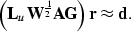
In order to achieve fast convergence, the modeling operator has to be as close to unitary as possible. Following the discussion in the preceding sections, we can define the pseudo-unitary operator as

$$\bold L_{u}=\bold L\bold W^{-\frac{1}{2}}$$ (15)

for which it is immediate to verify that $\bold L_{u}^{*}\bold L_{u}= {\bf I}$.

With this new operator, our least-squares problem may be rewritten as:

$$\left (\bold L_{u}\bold W^{\frac{1}{2}} \bold \AA\bold G\right )\bold r\approx \bold d.$$

We can redefine the model variable as a new, preconditioned variable

$$\bold p=\bold W^{\frac{1}{2}} \bold \AA\bold G\bold r,$$

which changes the optimization problem to the simple equation:

$$\bold L_{u}\bold p\approx \bold d.$$ (16)