The frequency domain approach

In contrast, the method developed by Herrmann et al. (2000) computes an approximation of the model covariance matrix in the Fourier domain. The main idea is to use the result of the inversion, as shown in equations (14) and (15), at one frequency as a weight for the next frequency. Consequently, this method takes advantage of the fact that the data are not aliased at low frequencies. Hence, the information from the lowest frequencies to the highest is transmitted and used to improve the focusing in the model space. I call this method the steering-weighting matrices method. It has the advantage of working noniteratively.

Taking this approach, starting from $\omega=\omega_{min}$ up to $\omega=\omega_{max}$, we begin with the two fitting goals for each frequency

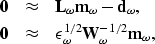$$\begin{eqnarray} {\bf 0} &\approx& {\bf L_{\omega}m_{\omega}-d_{\omega}}, \\ {\... ... \epsilon_{\omega}^{1/2} {\bf W}_{\omega}^{-1/2}{\bf m_{\omega}},\end{eqnarray}$$ (18) (19)

where the diagonal matrix ${\bf W}$ has components

$$W_{\omega}^{ii} = \vert \hat{m}_{\omega-1}^i \vert,$$ (20)

with ${\bf W}_{\omega_{min}}={\bf I}$.The division in equation (19) can be avoided if we use ${\bf W}_{\omega-1}^{-1/2}$ as a preconditioning operator Fomel (1997). Then, omitting the $\omega$, we obtain

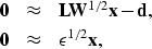$$\begin{eqnarray} {\bf 0} &\approx& {\bf LW}^{1/2}{\bf x-d}, \\ {\bf 0} &\approx& \epsilon^{1/2} {\bf x},\end{eqnarray}$$ (21) (22)

with ${\bf x = W}^{-1/2}{\bf m}$. The estimate of the model can be written as follows:  

$${\bf \hat{m}} = {\bf WL'}({\bf LWL'}+\epsilon{\bf I})^{-1} {\bf d},$$ (23)

or equivalently as  

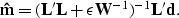$${\bf \hat{m}} = ({\bf L'L}+\epsilon{\bf W}^{-1})^{-1}{\bf L' d}.$$ (24)

Equation (23), used in the under-determined case, is clearly easier to compute because we do not have to calculate ${\bf W}^{-1}$. Since in practice we often have to deal with more unknowns than data points, I use equation (23) in the following examples.