Solving the Cauchy problem

 To obtain an explicit solution of the Cauchy problem (-) for equation (), it is convenient to apply the following simple transform of the wavefield P:  

$$P(t_n,h,y)=Q(t_n,h,y)\,t_n\,H(t_n)\;.$$ (287)

Here the Heavyside function H is included to take into account the causality of the reflection seismic gathers (note that the time t_n=0 corresponds to the direct wave arrival). We can extrapolate Q as an even function to negative times, writing the reverse of () as follows:  

$$Q(t_n,h,y)=Q(-t_n,h,y)=P(\vert t_n\vert,h,y)/\vert t_n\vert\;.$$ (288)

With the change of function (), equation () transforms to  

$$h \, {\partial^2 Q \over \partial y^2} = h\, {\partial^2 Q \... ...artial h} + t_n \, {\partial Q \over {\partial t_n}}\right) \;.$$ (289)

Applying the change of variables  

$$\rho={t_n^2 \over 2}\;,\;\nu={h^2 \over {2\,t_n^2}}$$ (290)

and Fourier transform in the midpoint coordinate y  

$$\widetilde{Q}(\rho,\nu,k)=\int\,Q(\rho,\nu,y)\,\exp (-iky)\,dy\;,$$ (291)

I further transform equation () to the canonical form of a hyperbolic-type partial differential equation with two variables:  

$${\partial^2 \widetilde{Q} \over {\partial \rho \, \partial \nu}} + k^2\,\widetilde{Q} = 0\;.$$ (292)

 

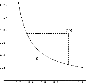
rim Figure 1 Domain of dependence of a point in the transformed coordinate system.

The initial value conditions () and () in the $\{\rho,\nu\}$ space are defined on a hyperbola of the form $\rho\,\nu=\left(h_1 \over 2\right)^2=\mbox{constant}$. Now the solution of the Cauchy problem follows directly from Riemann's method Courant (1962). According to this method, the domain of dependence of each point $\{\rho,\nu\}$ is a part of the hyperbola between the points $\{\rho,{h_1^2 \over {4\,\rho}}\}$ and $\{{h_1^2 \over {4\,\nu}},\nu\}$ (Figure ). If we let $\Sigma$denote this curve, the solution takes an explicit integral form:

$$\begin{eqnarray} \widetilde{Q}(\rho,\nu) & = & {1 \over 2}\, \widetilde{Q}(\rho,... ...\rho_1,\nu_1;\rho,\nu) \over {\partial \nu_1}} \right)\,d \nu_1\;.\end{eqnarray}$$ (293)

Here R is the Riemann's function of equation (), which has the known explicit analytical expression  

$$R(\rho_1,\nu_1;\rho,\nu)= J_0\left(2k\,\sqrt{\left(\rho_1-\rho\right)\, \left(\nu_1-\nu\right)}\right)\;,$$ (294)

where J₀ is the Bessel function of zeroth order. Integrating by parts and taking into account the connection of the variables on the curve $\Sigma$, we can simplify equation () to the form  

$$\widetilde{Q}(\rho,\nu)= \widetilde{Q}_0(\rho,\nu)+ \widetilde{Q}_1(\rho,\nu)\;,$$ (295)

where

$$\begin{eqnarray} \widetilde{Q}_0(\rho,\nu) & = & {\partial \over {\partial \rho}... ...l \widetilde{Q}(\rho_1,\nu_1) \over {\partial \nu_1}} \,d \nu_1\;.\end{eqnarray}$$ (296) (297)

Applying the explicit expression for the Riemann function R () and performing the inverse transform of both the function and the variables allows us to rewrite equations (), (), and () in the original coordinate system. This yields the integral offset continuation operators in the $\{t_n,h,k\}$ domain  

$$\widetilde{P}(t_n,h,k)= H(t_n)\,\left(\widetilde{P}_0(t_n,h,k) + t_n\,\widetilde{P}_1(t_n,h,k)\right)\;,$$ (298)

where

$$\begin{eqnarray} \widetilde{P}_0 & = & {\partial \over {\partial t_n}}\, \int_{... ...}\right)\, \left(t_n^2-t_1^2\right)}\right)\,{dt_1 \over t_1^2}\;,\end{eqnarray}$$ (299) (300)

$$\begin{eqnarray} \widetilde{P}^{(j)}_1(t_1,k) & = & \int\,P\,^{(j)}_1(t_1,y_1)\... ...lde{P}(t_n,h,k) & = & \int\,P(t_n,h,y)\exp (-iky)\,dy\;(j=0,1)\;.\end{eqnarray}$$ (301) (302)

The inverse Fourier transforms of equations () and () are reduced to analytically evaluated integrals Gradshtein and Ryzhik (1994) to produce explicit integral operators in the time-and-space domain  

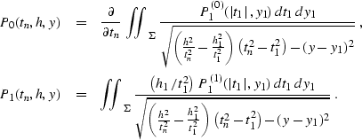
$$P(t_n,h,y)=\mbox{sign}(h-h_1)\, {H(t_n) \over \pi}\,\left(P_0(t_n,h,y) + t_n\,P_1(t_n,h,y)\right)\;,$$ (303)

where

$$\begin{eqnarray} P_0(t_n,h,y) & = & {\partial \over {\partial t_n}}\, \iint_{\S... ..._1^2 \over t_1^2}\right)\, \left(t_n^2-t_1^2\right)-(y-y_1)^2}}\;.\end{eqnarray}$$ (304) (305)

The range of integration $\Sigma$ in () and () is defined by the inequality  

$$\left({h^2 \over t_n^2}-{h_1^2 \over t_1^2}\right)\, \left(t_n^2-t_1^2\right)-(y-y_1)^2 \gt 0\;.$$ (306)

Equations (), (), and () coincide with (), (), and () in the main text.