Test example

For a simple 1-D test of B-spline regularization, I chose the function shown in Figure , but sampled at irregular locations. To create two different regimes for the inverse interpolation problem, I chose 50 and 500 random locations. I interpolated these two sets of points to 500 and 50 regular samples, respectively. The first test corresponds to an under-determined situation, while the second test is clearly over-determined. Figures 23 and 24 show the input data for the two test after normalized binning to the selected regular bins.

 

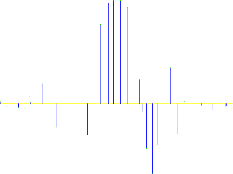
bin500 Figure 23 50 random points binned to 500 regular grid points. The random data are used for testing inverse interpolation in an under-determined situation.

 

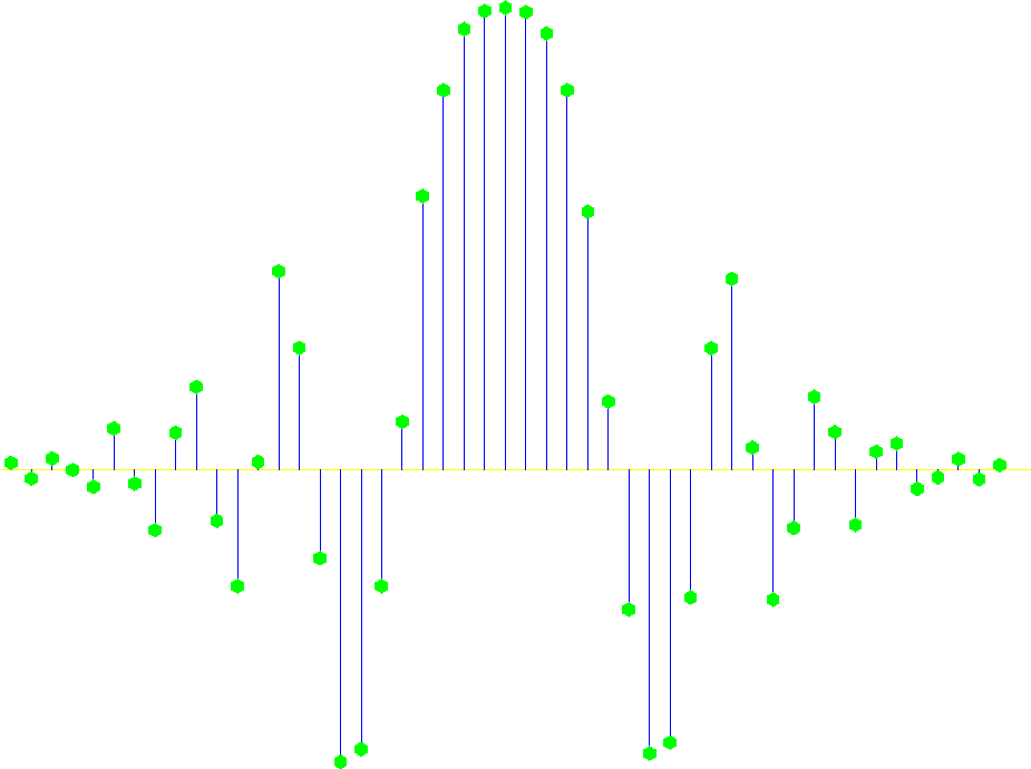
bin50 Figure 24 500 random points binned to 50 regular grid points. The random data are used for testing inverse interpolation in an over-determined situation.

I solved system (12)-(18) by the iterative conjugate-gradient method, utilizing a recursive filter preconditioning for faster convergence. To construct the regularization operator $\bold{D}$, I used the method of the previous subsection with the tension-spline differential equation that I will describe in Chapter .

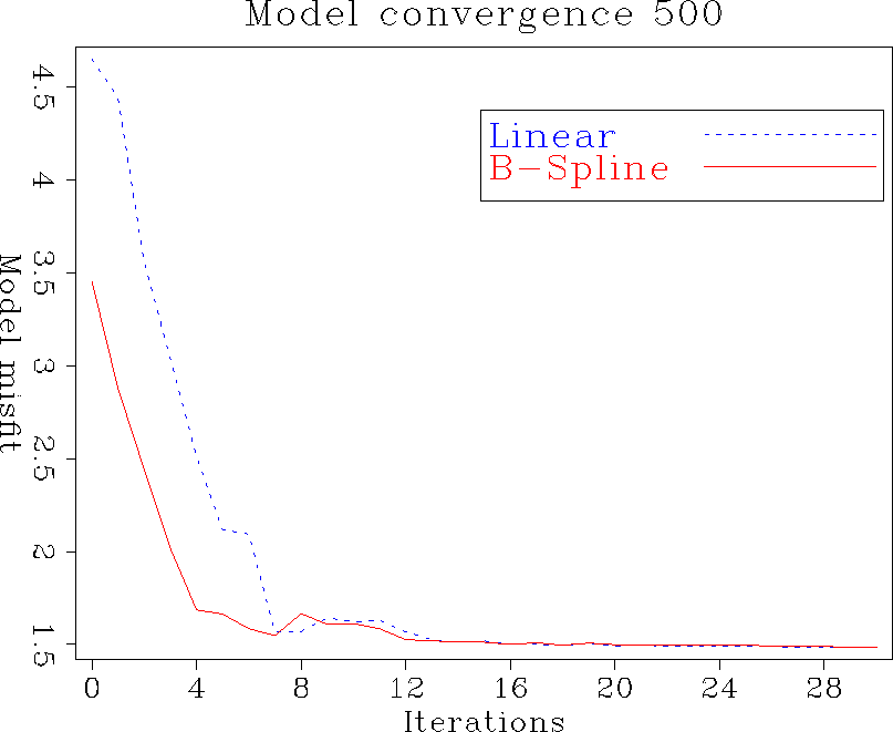
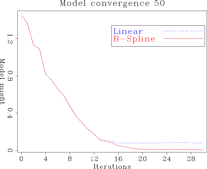
The least-squares differences between the true and the estimated model are plotted in Figures 25 and 26. Observing the behavior of the model misfit versus the number of iterations and comparing simple linear interpolation with the third-order B-spline interpolation, we discover that

• In the under-determined case, both methods converge to the same final estimate, but B-spline inverse interpolation does it faster (with fewer iterations). However, the total computational gain is not significant because each B-spline iteration is more expensive than the corresponding linear interpolation iteration.
• In the over-determined case, both methods converge similarly at early iterations, but B-spline inverse interpolation results in a more accurate final estimate.

From the results of this simple experiment, it is apparent that the main advantage of using more accurate interpolation in the data regularization context occurs in the over-determined situation, when the estimated model is well constrained by the available data.

 

norm500 Figure 25 Model convergence in the under-determined case. Dashed line: using linear interpolation. Solid line: using third-order B-spline.

 

norm50 Figure 26 Model convergence in the over-determined case. Dashed line: using linear interpolation. Solid line: using third-order B-spline.