Tomography and null space

If the model space is a uniformally sampled Cartesian mesh or something similar, we face another problem when doing reflection tomography, its large null space. There are several reasons for this null space:

shadow zones

Certain parts of the velocity model simply might not be illuminated, or illuminated poorly by the acquisition geometry. A classical example is under the edge of a salt body ().

limited angle coverage

The recording geometry imposes a limitation on vertical resolution. The left panel of Figure 5 simulates a ray-based back projection operator. Along each ray a random slowness change is back projected. The right panel of Figure 5 shows the Fourier response. Note how large wavenumbers in z are not well illuminated. Often this phenomenon is explained in terms of the Fourier slice theorem. The Fourier transform of a vertical projection in space is a horizontal radial profile.

 

slice
Figure 5 The left panel simulates a ray-based back projection operator. Along each ray a random slowness change is back projected. The right panel shows the Fourier response.

resolution decreases with depth

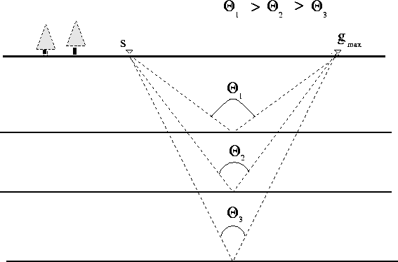
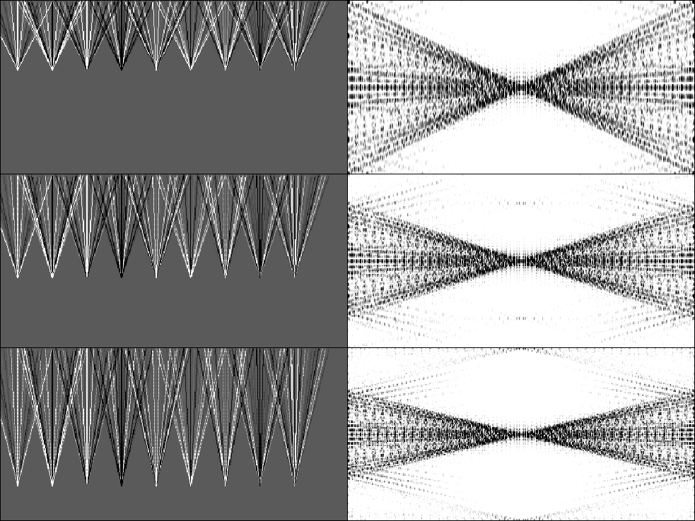
When the reflection point is unknown, normal angle reflection times do not contain any information about velocity. As the reflection angle increases, velocity discrimination becomes easier. At larger depths, given the limited surface recording geometry, the angle coverage will decrease (Figure 6). As a result, larger depth model components are often under- or unilluminated (). If we follow the Fourier analysis of Figure 5 we can see that the vertical resolution decreases as the reflector depth increases (Figure 7).

 

ray-limit Figure 6 Given a fixed recording geometry (s being the source and $g_{\rm max}$ being the farthest receiver) as we go deeper in depth the angle range that we at each reflector decreases.

 

slice.depth
Figure 7 Left panel shows simulated raypaths with random energy introduced along each raypath. The right panel is the Fourier response. From top to bottom the depth of the reflector increases.

not enough equations

In most reflection tomography methods, we invert a limited set of positioning errors. When doing tomography, especially 3-D tomography, it is possible to have more model points than moveout errors.

To deal with the null space of the reflection tomography operator there are two alternative paths that could be followed, reparameterization or regularization.

Reparameterization can be done by a coarser sampling of the Cartesian, but usually involves other parameterizations of the model space. It usually takes the form of either a layered model with simple velocity function (such as velocity gradient) within the layers () or reparameterizing the model in term of spline nodes (). The layered model approach is attractive because it allows a linking between an interpreter's geologic model (). It also provides a fairly accurate description of velocity structure in regions such as the North Sea. The spline node approach can also be beneficial. It can guarantee the velocity model will be smooth (necessary for ray based methods) and with selective placement of nodes can allow less freedom in areas where the data provides less information about the velocity field. The downside of both of these approaches is that the parameterization must be chosen a priori. At early iterations the guess at the velocity model can be in significant error. If we do a poor job of parameterizing the model we could actually slow, or stop, the problem from converging ().

The second option is regularization. In the regularization approach we add a second term to the objective function,

(4)

where $\bf A$ penalizes some definition of roughness in the model. The regularization approach has its own drawbacks. The most significant is that the resulting model space may no longer has any direct connection with geology. In addition, choosing $\bf A$ is problematic and can introduce unrealistic elements into the slowness estimate.