Tomography, or at least the definition of tomography I will
be using in thesis, starts from
the idea that there is an operator
![]() that relates slowness
that relates slowness ![]() to travel times ,
to travel times ,
| (1) |
|
cor.overlay
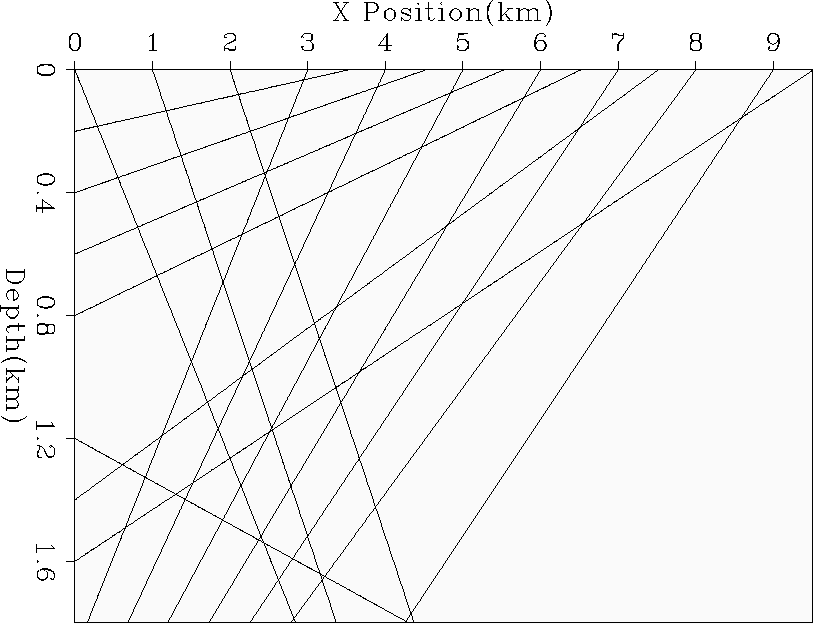
Figure 1 A simple example of tomography with the sources and receivers every .2 km in depth and every .5 km in x. Overlaid are the raypaths connecting the sources to the receivers. |  |
This simplistic view of tomography has a number of inconsistencies
with the reflection tomography problem.
The first is that we wouldn't be doing tomography
if we actually knew the slowness field beforehand.
What we actually have is some initial guess, ![]() , of the slowness field.
If for our initial model
we assume a constant slowness field and find the raypaths connecting the
same source and receivers,
Figure 2, we encounter
another problem: the raypaths are significantly different. An alternate
way to state this observation is that the operator is model dependent
and therefore non-linear.
, of the slowness field.
If for our initial model
we assume a constant slowness field and find the raypaths connecting the
same source and receivers,
Figure 2, we encounter
another problem: the raypaths are significantly different. An alternate
way to state this observation is that the operator is model dependent
and therefore non-linear.
|
init.overlay
Figure 2 The same recording geometry as Figure 1, with a constant velocity field. Note that the ray paths are significantly different. |  |