Marine 3-D shot interpolation example

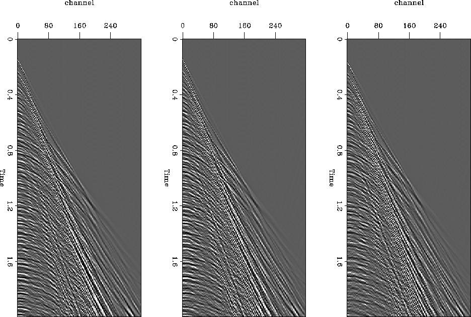
Figure curt.in shows another shot gather, this from one a 3-D marine survey. While in previous examples I threw out portions of a 2-D survey, to simulate a flip/flop acquisition, this data actually was collected with a flip/flop acquisition. Thus we can not do exactly the same experiments as with the previous 2-D examples. On the other hand, the dips in this data are more routine than those in the previous data, so it should be subsampled more to make an interesting test. Instead we start from the slightly subsampled data (using one source from a two-source survey), and remove half the shots again, so the shot interval is four times the receiver interval.

Figure curt.in shows one of the shot gathers that was removed, and the interpolated version of that shot gather is shown in Figure curt.out. The interpolated shot gather is extremely faithful to the original, predicting 94% of its variance. The most noticeable differences are back-scattered noises at late times and short offsets which are not interpolated well. In the electronic version of this document, Figure curt.in is a two-frame movie, comparing the original and interpolated gathers.

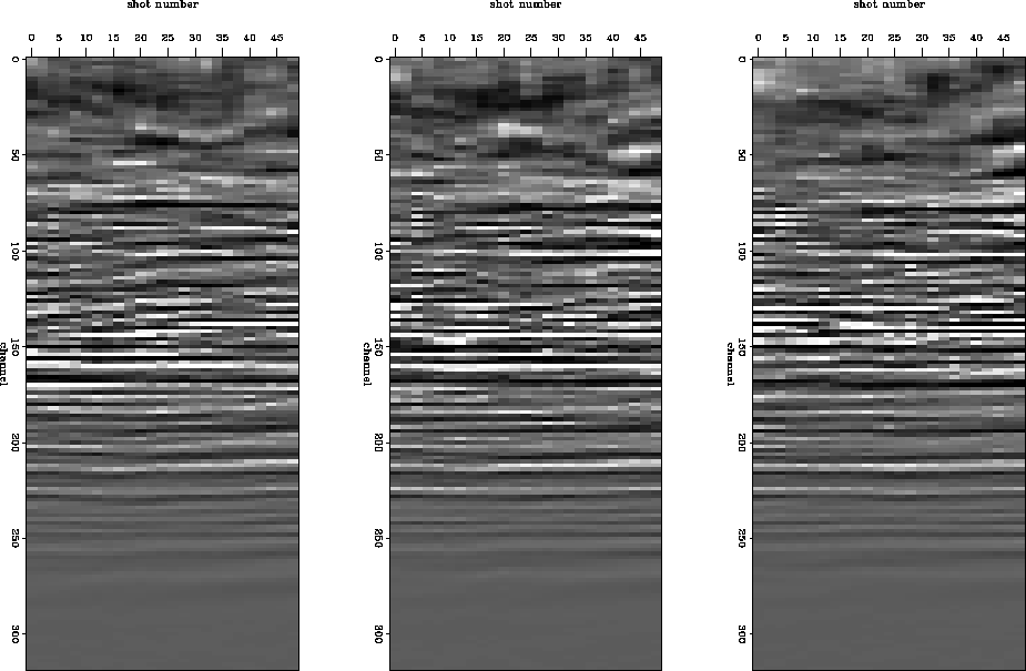
Figures curt.in.ts and curt.out.ts show another view. These are time slices through cubes made up of one source and one streamer. The three slices in each figure correspond to the three steamers in the survey. Not surprisingly, the time slices appear slightly smoothed along the shot number axis, where the data were subsampled. The visible events are all continued in a coherent manner, but may be a bit too coherent in areas where some high-wavenumber fluctuations of events were removed by the subsampling, and then replaced in a smooth fashion by the interpolation.

 

curt.in
Figure 10 3-D shot gather. This shot gather was among the half removed from the input data, and then reinterpolated. The interpolated version of this shot gather is shown in Figure curt.out.

 

curt.out
Figure 11 Recreated 3-D shot gather. The shot gather in Figure curt.in was removed and interpolated from nearby shots to produce this shot gather.

 

curt.in.ts
Figure 12 Time slice from a 3-D survey. This is a slice through a cube made up of shots from one of two sources, and receivers from three streamers. Each panel corresponds to one streamer.

 

curt.out.ts
Figure 13 Recreated time slice from a 3-D survey. Every second shot from the data shown in Figure curt.in.ts was removed and then reinterpolated. This time slice is from the interpolated cube, at the same time sample as above.