Marine 2-D shot interpolation example

Figure 355exshotgather shows a slice from a cube of 2-D shot gathers. The data have long-period multiples, and complicated moveouts caused by a tabular salt body. The geologic structure in the area is similar to the model used to generate the synthetic data in the previous chapter, though this data has the virtue and added complications of being real field data. This data set is 2-D, with shot sampling and receiver sampling equal. As in the last chapter, we can throw out alternating receivers in a checkerboard pattern to simulate common receiver gathers formed from a single inline from a 3-D survey with flip/flop acquisition. We can also just throw out alternating shots to simulate common shot gathers from the same survey.

 

355exshotgather
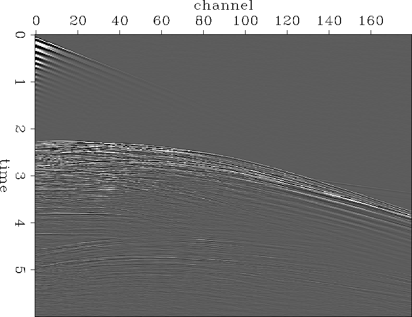
Figure 6 Sample shot gather from the original data.

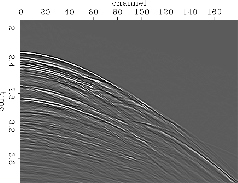
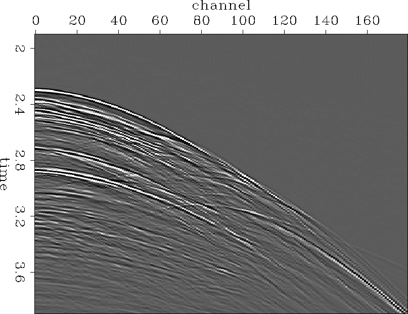
As a test, we interpolate both ways. Figure 355start.shot shows a closeup of the input, zoomed in on regions between 2 and 4 seconds in Figure 355exshotgather. Figure 355shotsub.out.shot shows the interpolation result on common shot gathers. Figure 355recsub.out.shot shows the interpolation result on simulated common receiver gathers. The traces shown in Figure 355recsub.out.shot are the same as in the other figures, but traces were zeroed in a checkerboard pattern (as in Figure traces-crg) to simulate the pattern of known and missing traces that arises from forming common receiver gathers after throwing out every second shot. In the other case, where the data are just representing shot gathers, every second slice in the cube was zeroed (as in Figure traces-csg).

 

355start.shot Figure 7 Portion of a marine shot gather. Part of the original data that is subsampled and interpolated to make the next figures.

 

355shotsub.out.shot Figure 8 Portion of an interpolated marine shot gather. This is the result of subsampling the shot axis and interpolating with the data sorted as shot gathers.

 

355recsub.out.shot Figure 9 Portion of an interpolated shot gather. This result simulates subsampling the shot axis and interpolating with the data sorted as receiver gathers.

The most obvious difference between the results in Figures 355shotsub.out.shot and 355recsub.out.shot is in the events which dip back towards zero offset. The data which are interpolated in slices have lost most of these events, while the data which are interpolated in the checkerboard pattern restored those somewhat. In the best case, just under 95% of the variance of the original data is predicted.

An unexplored alternative to resorting the data may be to rotate the filters by 45 degrees.