 |
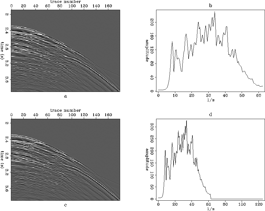
Figure 9 Samples of input data. The panels show (a) 8 ms input data and (b) its power spectrum; and (c) 4 ms input data and (d) its power spectrum.
Dips do not change when the PEF's axes are scaled, but frequencies do. This has two important consequences. The first relates to the data's temporal nyquist. The filter that we calculate, shown in Figure exp, has half the temporal Nyquist of the filter in Figure 3dpef. So even though seismic data is almost never temporally aliased, we can have a problem estimating filter coefficients if the data contains frequencies above the half-Nyquist. Components at certain dips and frequencies will simply slip through the gaps in the axis-scaled filter, and be effectively invisible.
This is not a problem in principle, because since the data are not temporally aliased, it is easy to resample the time axis and make sure the signal is below the half-Nyquist. But it is something that is important to remember in practice. Figures nyqin and nyqout show an example of the difference that resampling can make. Figure nyqina shows a slice from a small cube of seismic data, bandpassed and sampled at 8 ms so that the data band just fills all the available frequencies, and Figure nyqinb shows its power spectrum. Figure nyqinc shows the same data, resampled to 4 ms so that the data band fills half the available frequencies, with zeroes above the half-Nyquist, and Figure nyqind shows its power spectrum. Neither dataset is temporally aliased. Figure nyqout shows results of zeroing half the traces in those two inputs, and then interpolating to fill the zeroed traces back in. The 8 ms data gives a poor interpolation result, shown in Figure nyqouta. In some areas it is fine, and in some it is terrible. The badly interpolated regions correspond to areas where a significant component of the data slips through the gaps in the axis-scaled filter. The 4 ms data (with signal at or below the half-Nyquist) produces a good result, shown in Figure nyqoutb.
 |
 |
So this is a manageable issue, but it does have some important consequences later, particularly with regards to sorting the input data. In particular, it is not hard to think of a situation where you would rather interpolate to a sampling three or four times denser than the input, rather than double as in most of the examples in this thesis. It is easy enough to scale the filter's axes by three or four, but that requires more resampling of the time axis, to be sure that the filters do not miss the higher frequencies in the data. That in turn requires many more filter coefficients to cover the same range of slopes in the data. Too many filter coefficients (degrees of freedom) is often a problem. In fact, even with very low frequency input, my experience has been that results turn out to be better when the data are interpolated in several smaller steps, rather than one large step. An example is shown in the next chapter.
A second potential problem associated with scaling the PEF's axes relates to dispersive data. Scaling PEF axes assumes that events lie along lines in Fourier space, so that time dip is independent of frequency. Dispersive waves have velocities which vary with frequency. If the slope (velocity) of a seismic event is different at different frequencies, then the data's PEF at one scale may not predict that data at a different scale. In real data examples, I have not found it to be a noticeable problem. Ground roll is dispersive, but can typically be interpolated. An illustration of the potential problem, and the reason it may not be a serious issue in real data, is shown in Figure disp2.
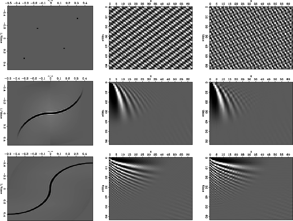
Figure disp2 shows three data sets with dips varying with frequency. Each row shows a data set's 2-D Fourier transform, original time-domain data, and the result of subsampling and then interpolating the data.
In the first example, the data are just two sinusoids with different frequencies. It seems to be a simple example to interpolate, but the result in the top right panel is terrible. The estimated PEF's spectrum needs to match the data at only a few points in Fourier space, and those points effectively move when the filter is rescaled. The result is interpolated data with the wrong dips.
The second and third examples are synthetics intended to simulate dispersive waves. In these cases, time dip of the events is a smooth function of their frequency. The interpolations are somewhat successful, though not perfect (as we would hope on a simple, noise-free synthetic). The example in the second row uses a single PEF, the example in the bottom row uses nonstationary PEFs. The example in the bottom row is harder because the amplitude in Fourier space does not decrease noticeably as the event bends. A single filter does not produce a good interpolation result in that example. Using multiple filters is effectively just a way to take some of the curvature out of Fourier space. In the middle row example, the energy dies off more quickly as the event curves.
 |
Parenthetically, this example also points out that the interpolation process as a whole is nonlinear in the amplitude of the data, though the two individual steps of least squares are both linear. For instance, in the top row, the input data is the combination of two data sets, each with a single dip. Either of the two can be interpolated perfectly by itself. This is an issue if we think of starting from a nonzero solution for the missing data samples. Something like linear interpolation might seem to be a sensible way to get an initial guess, but Figure introex points out that that is not going to be useful if the data are not already well sampled. Nonlinearity adds the prospect that linear interpolation or some other simple method may ultimately worsen the result.