Nonstationarity

The theory in this chapter assumes that the data are wide-sense stationary. A data sequence is considered to be wide-sense stationary if it has constant mean and if its autocorrelation is strictly a function of lag  

$$E\left[ u(n_1)u(n_2) \right] = a(n_1,n_2) = a(n_1-n_2)$$ (22)

Throughout this thesis, when data are said to be stationary, I mean that they are wide-sense stationary. This is as opposed to strict-sense stationary, which means that the data have the same probability mass function everywhere.

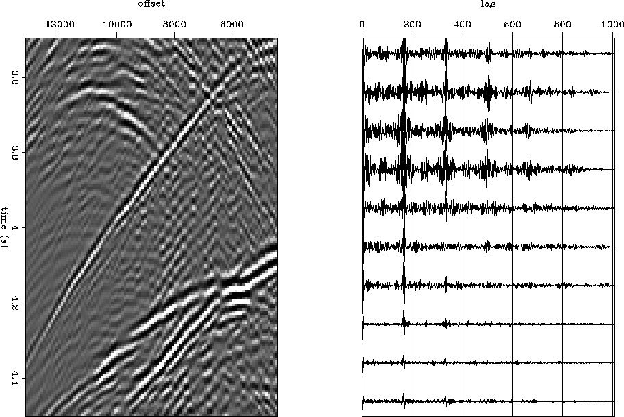
We want to look at data with more than one dimension. Thinking in helical coordinates, we can view a set of traces as a super trace and take its autocorrelation. Equation station says that we should be able to get the same autocorrelation function for different subsets of the data (different starting samples n₁). Intuitively, this coincides with the statement in the introduction (taken from Spitz 1991) that the data should be made up of linear events of constant slope. Figures stationdata and nonstationdata show examples. Figure stationdata shows a window from the far offsets of a synthetic CMP gather, and autocorrelation sequences made from identical numbers of samples, starting at different places within the window. Figure nonstationdata shows a window from the inner offsets of the same gather, and autocorrelation sequences. The far offsets, where data tends to be made up of linear events as hyperbolas approach their asymptotes, are by appearance nearly stationary, and the autocorrelations are approximately equal except for a scale factor. The inner offsets, where the events are obviously changing dip, do not look stationary and do not have approximately equivalent autocorrelation functions.

 

stationdata
Figure 12 Synthetic seismic data, and autocorrelation functions calculated from different subsets of the data. The data are approximately wide-sense stationary, so the autocorrelations are approximately identical, except for a scale factor.

 

nonstationdata
Figure 13 Synthetic seismic data, and autocorrelation functions calculated from different subsets of the data. The data are nonstationary, so the autocorrelations are significantly different.

Seismic data are not, as a rule, stationary. The slopes of seismic events change with offset and time, and when the geology is nontrivial, with surface locations also. This just means that we can not use a single PEF to represent the spectrum of all the data, but only as much data as we can reasonably assume to be stationary.