 |
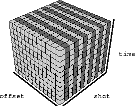
Figure 4 Arrangement of recorded and missing traces in one inline of a dual-source marine experiment, sorted into common receiver gathers. One shade represents recorded traces and the other missing traces.
The PEF that minimizes the causal prediction error turns out to have the inverse of the data spectrum as its spectrum. With such a filter, Claerbout's statement at the beginning of this chapter tells how to then fill in the missing traces. However, interpolation is interesting only when the data are aliased. And when the data are aliased, the data spectrum is not really a sensible choice. The data aliasing is expressed in the Fourier domain by the wraparound artifacts, which need to be unwrapped for the interpolation to be useful. Otherwise, we could do everything instantly in the Fourier domain by zero padding or something similar, and not bother with filter estimation at all. This complication turns out to illustrate another important PEF property, scale invariance.
The data that we use to calculate PEFs is incomplete. We can imagine the missing traces that we want to eventually fill in as being composed of zeroes. We can rearrange the recorded data and the zeroes in various ways by sorting the data. Continuing with the idea of missing shots in marine acquisition, we can sort the data into common receiver gathers and form a checkerboard of recorded and zero traces, as shown in Figure traces-crg. We can choose to leave them as shot gathers, and have the arrangement shown in Figure traces-csg.
 |
 |
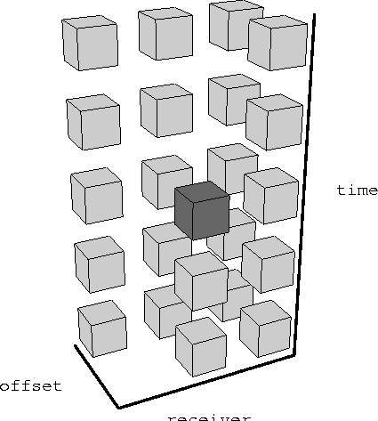
We do not want those zeroes to influence our filter estimation, so we scale the axes of the filter. Figure exp shows the PEF from Figure 3dpef, but with all its axes scaled by two. Again the dark box is the fixed 1 and the lighter boxes hold the adjustable coefficients. The empty spaces between boxes are lags with no coefficients in them. Convolving the filter in Figure 3dpef across either of the data cubes in Figures traces-crg and traces-csg results in predicting zeros from known data values, or known data values from zeros, depending on the position of the filter in the data cube. Convolving the filter in Figure exp across the same data cubes results in predicting zeros from zeros, or known data from known data only. That is what we want. The PEF should find the spectrum of just the recorded data.
|
exp
Figure 6 A 3-D prediction error filter with all axes scaled by two. |  |
All the axes are scaled equally. It looks as though we only need to scale the spatial axes. However, if we only scale the spatial axes, then the dips represented by the original-size filter (Figure 3dpef) will not be the same as the dips represented by the scaled filter (Figure exp). We need to return the filter to its original size in order to fill in the missing traces. As an aside, scaling the filter halves the temporal Nyquist of the filter. If the input data contain frequencies above the half-Nyquist, it is important to resample the time axis. This is discussed in more detail later.
Calculating data values to put in the missing traces
is exactly like calculating filter coefficients.
Minimize the mean square of the prediction error
![]() , except instead of changing the filter coefficients a(n),
change the data values u(n).
Naturally the recorded data should not change, so change
only the u(n) that were not part of the original data set,
those corresponding to the zero traces in Figures
traces-crg and traces-csg.
, except instead of changing the filter coefficients a(n),
change the data values u(n).
Naturally the recorded data should not change, so change
only the u(n) that were not part of the original data set,
those corresponding to the zero traces in Figures
traces-crg and traces-csg.
The filter with scaled axes, shown in Figure exp, does not predict missing values from known ones, so there is no criteria for assigning values to the missing data. In order to move energy between the known and missing traces, we rescale the axes so that the filter is compressed to its original size, as in Figure 3dpef. Happily, the PEF's wrapped (aliased) spectrum that is calculated from the aliased data seems to come unwrapped; depending on how aliased the original data is, the rescaled filter is less aliased or not aliased at all. The PEF coefficients were calculated so that the PEF's spectrum was the inverse of the data spectrum. By the same method, the adjustable data values are calculated to have the inverse of the PEF spectrum, which is just the original data spectrum again, but with aliasing wrap-around removed. Where before the filter took on the inverse of the aliased data spectrum, now the data takes on the inverse of the unaliased filter spectrum.
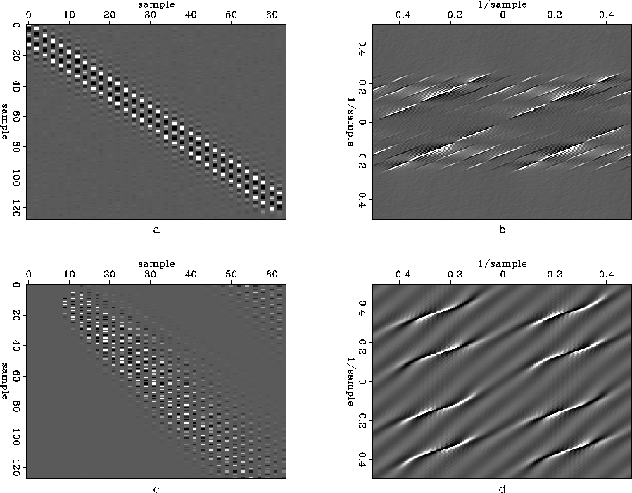
As an example, Figures diagonalin2 and diagonalout2 show a simple diagonal example similar to the one in the introduction. Figure diagonalin2 shows the aliased input data (diagonalin2a), its Fourier transform (diagonalin2b), the impulse response of the inverse of the axis-scaled PEF calculated from the data (diagonalin2c), and the Fourier transform of that (diagonalin2d). The axis-scaled PEF whitens the aliased input data, knocking down the dominant events in the data. Accordingly, the same four strong events are visible in the spectrum of the input and of the inverse PEF. Oddly enough, the inverse PEF has some additional events in its spectrum, at high frequencies where the data spectrum is all zero. The inverse PEF is the estimate of the spectrum of the data, so it seems strange to see energy where the data spectrum is known to be zero. However, those components of the model (the PEF) are in null space of the operator (convolution with the data), since multiplying anything by the zeroes in the data spectrum gives zero.
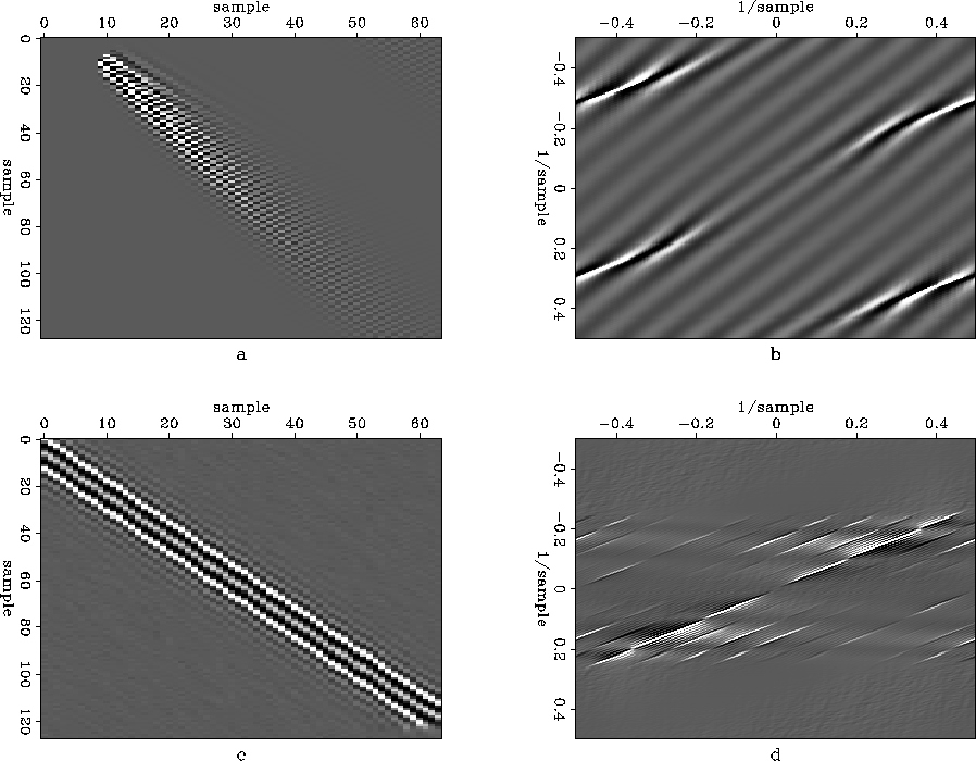
Figure diagonalout2 shows the impulse response of the inverse PEF with its axes returned to normal size (diagonalout2a), the Fourier transform (diagonalout2b), the interpolated data (diagonalout2c), and the interpolated data's Fourier transform (diagonalout2d). When the PEF is compressed to normal size, its spectrum is windowed down to a less-aliased region, which parenthetically happens to get rid of those surprising high-frequency events in the PEF. The interpolated data then takes on the spectrum of the compressed PEF. There is still an obvious alias in this particular PEF's spectrum, but it again is outside the band of the data.
 |
 |