|
synt-bob
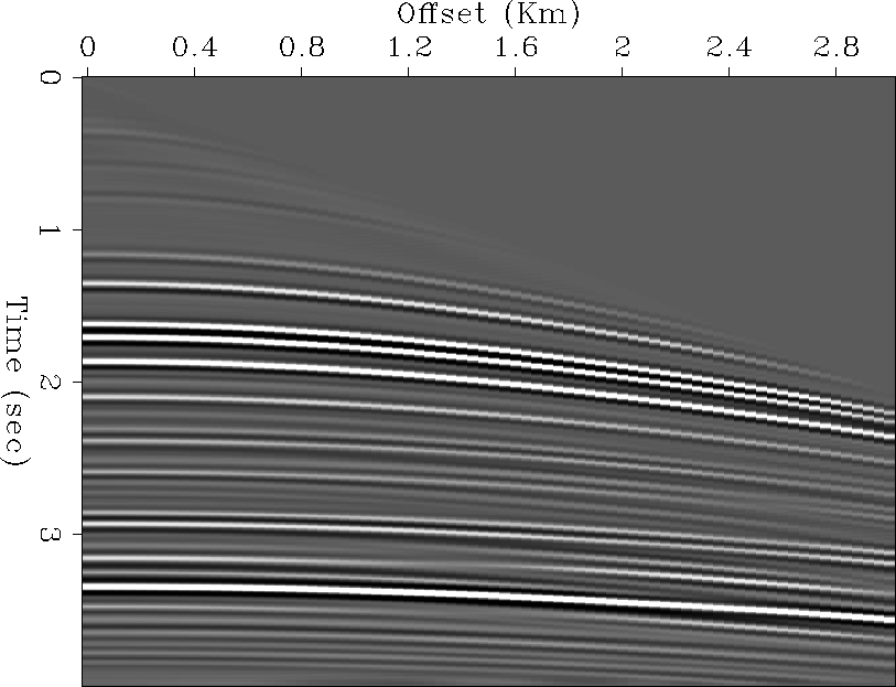
Figure 1 Synthetic Model. |  |
A synthetic interval velocity model was built and a CMP gather was modeled using a finite difference code (Figure 1)
|
synt-bob
Figure 1 Synthetic Model. |  |
For this gather, a velocity analysis is performed to obtain the RMS
velocity ![]() (equation 1).
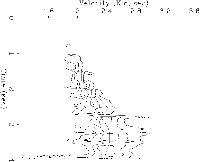
Figure 2 shows the rms velocity
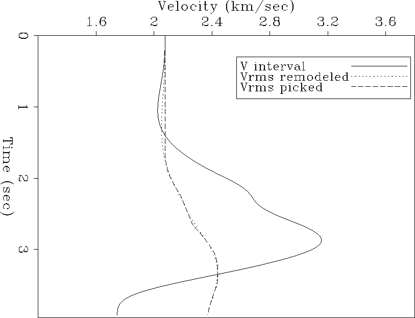
curve picked from the data, and Figure 3 shows
a comparison of
the interval velocity
(equation 1).
Figure 2 shows the rms velocity
curve picked from the data, and Figure 3 shows
a comparison of
the interval velocity ![]() obtained by the methodology
described above, the RMS velocity
obtained by the methodology
described above, the RMS velocity ![]() obtained from
the velocity analysis, and the remodeled RMS velocity (
obtained from
the velocity analysis, and the remodeled RMS velocity (![]() =
=
![]() ).
).
This comparison shows that the remodeled RMS velocity is similar to the picked RMS velocity. This similarity prove that the method used works well.
|
scan-bob
Figure 2 Velocity analysis for the first synthetic example. The curve corresponds to the picked RMS velocity |  |
|
compar-bob
Figure 3 Comparison of interval and RMS velocities. |  |