Example

In this section, I present a synthetic example of Stolt migration and residual migration for common-azimuth data. The model is represented by a set of four plane reflectors at different depths, with different lateral dimensions and varying reflectivity (Figure 1).

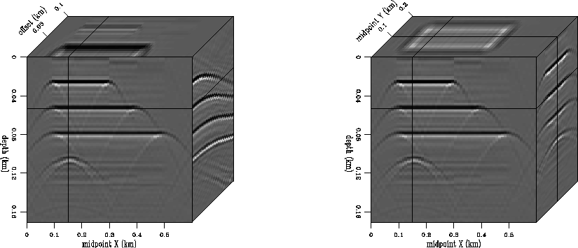
Figure 2 shows the result of Stolt modeling using the true velocity v=3.0 km/s. Next, I apply Stolt migration with a velocity of v₀=3.6 km/s (Figure 3). Since the velocity is not the true one used to generate the data, the image is not focused correctly at the three original reflectors.

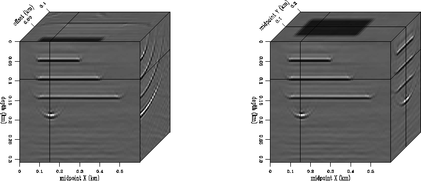
Finally, I use Stolt common-azimuth residual migration as described in the preceding section and with a velocity ratio v₀/v=1.2 to get the image in Figure 4. Now the original reflectors are well-focused at their original locations.

 

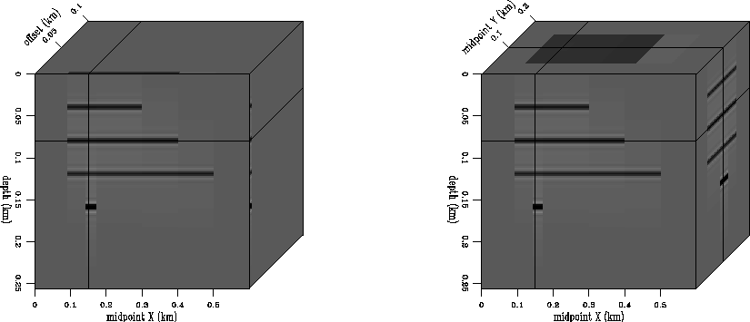
model
Figure 1 The reflectivity model. The right panel represents the zero-offset view in the common-azimuth space, while the left panel represents the prestack view for the inline selected on the right panel.

 

data
Figure 2 The data generated using Stolt common-azimuth modeling. The velocity used for modeling is v=3.0 km/s. The right panel represents the zero-offset view in the common-azimuth space, while the left panel represents the prestack view for the inline selected on the right panel.

 

mig
Figure 3 The image obtained using Stolt common-azimuth migration. The velocity used for migration is v₀=3.6 km/s. Since v₀ > v, the image is clearly over-migrated. The right panel represents the zero-offset view of the common-azimuth data, while the left panel represents the prestack view for the inline selected on the right panel.

 

rst
Figure 4 The image obtained using Stolt common-azimuth residual migration using velocity ratio v₀/v=1.2. The image is nicely focused at zero-offset. The right panel represents the zero-offset view of the common-azimuth data, while the left panel represents the prestack view for the inline selected on the right panel.