


This section discusses practical issues for a cost-effective implementation of AMO as an integral operator in the time-space domain. The main challenge is to take advantage of the limited aperture for the integration to save computational costs while avoiding operator aliasing. For small azimuthal rotations, the saddle describing the AMO impulse response has a strong curvature that requires special handling of operator antialiasing. The trick is to perform the spatial integration in a transformed coordinate system where the AMO surface becomes invariant with respect to the amount of azimuth rotation and offset continuation. The appropriate midpoint-coordinate transformation is described by the following chain of transformations Fomel and Biondi (1995b):
| (5) |
 |

In this new coordinate system, the kinematics of AMO are described by the following simple relationship between the input time t1 and the output time t2
| (6) |
and the amplitudes (based on Zhang-Black amplitudes for DMO) are described by the following equation
| (7) |
which takes into account the Jacobian factor introduced by the coordinate transformation.
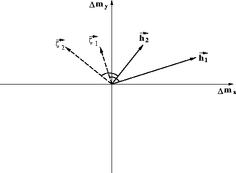
To avoid operator aliasing, one should apply a low-pass filter whose bandwidth varies spatially along the operator and is a function of the local time dips of the operator. The time dips can be computed analytically according to the following equations:
 |
(8) | |
| (9) |
Finally, and taking into account the dependency of the AMO aperture on velocity, the maximum output time can be evaluated for a given minimum propagation velocity Vmin as
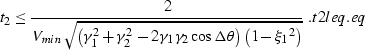 |
(10) |
where ![]() and
and ![]() are given by
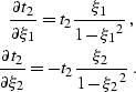
are given by
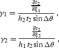 |
(11) | |
| (12) |
To avoid truncation artifacts, a tapering function should be applied to the edges of the operator aperture.