Deconvolution Examples

The operator A is 1D convolution of a source pulse w with the input time series x. The data d is this convolution plus the noise series n. The regularization operator R is taken to be the identity I for all examples presented here.

All of the examples in this section will concern the source pulse (w) depicted in Figure 1, which is a 15 Hz Ricker wavelet sampled at 4 ms.

 

fig1 Figure 1 15 Hz Ricker wavelet used in deconvolution experiments.

The data space consists of time series of length 1001, sample rate 4 ms. The noise free data is the convolution of the wavelet with a spike located at 1 s, see Figure 2.

 

fig2 Figure 2 Noise free data.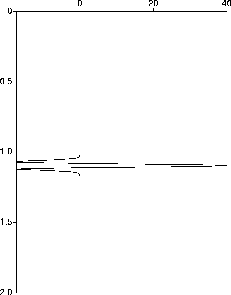

The noise strength for the first set of experiments is 0.5. The noise is concentrated in the pulse passband, as it is the convolution of a pseudorandom sequence with the pulse, followed by scaling. Thus a signal of reasonable size fits the noisy data (Figure 3) very precisely.

 

fig3 Figure 3 Noisy data: 50% RMS filtered noise.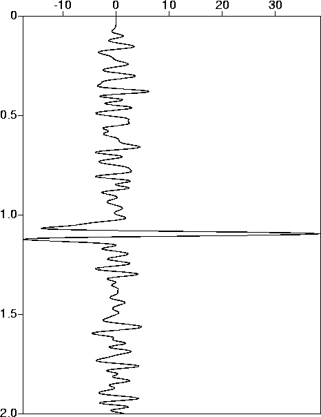

The deconvolutions (signal estimations) resulting from underestimating, correctly estimating, and overestimating the noise level appear as Figure 4, Figure 5, and Figure 6. The estimated noise levels are 10%, 50%, and 80% respectively. In the notation of the last section, $\sigma =$0.1, 0.5, and 0.8 respectively. There is no particular identifiable virtue of one result over the other, which reinforces my contention that in order to solve one of these problems, you must have an independent means of estimating noise level: neither the data nor the results of the signal estimations reveal the signal/noise dichotomy.

 

fig4 Figure 4 Signal estimate: target noise level 10%, filtered noise.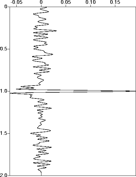

 

fig5 Figure 5 Signal estimate: target noise level 50%, filtered noise.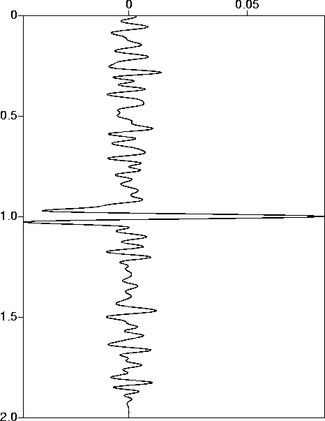

 

fig6 Figure 6 Signal estimate: target noise level 80%, filtered noise.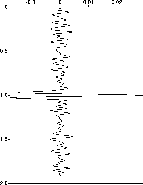

Note that even for the correctly estimated noise level, namely $\sigma = 0.5$, you do not recover the isolated spike. The discrepancy is partly due to the less than perfect linear system solves via conjugate gradient iteration, but also to the nature of the problem: it is actually possible to achieve the same fit error as that provided by the noise free data with a slightly smaller signal, by fitting the signal less and the noise more. That's because signal and noise are not entirely orthogonal (and they rarely are, so you're going to have to live with this ``crosstalk'' imperfection!).

The relation between the noise level or fit error and the penalty parameter $\epsilon$ really is obscure, as the following results suggest:

• $\sigma =$ 0.1 $\Rightarrow \epsilon =$ 50.9061
• $\sigma =$ 0.5 $\Rightarrow \epsilon =$ 210.593
• $\sigma =$ 0.8 $\Rightarrow \epsilon =$ 459.234

I would not have guessed the precise values of these $\epsilon$s - would you have done? On the other hand the trend is exactly as you would expect: as you permit more misfit, you are able to make the auxiliary quantity (the model L² norm in this case) smaller, corresponding to a larger $\epsilon$.

The second set of experiments uses the same noise free data contaminated with unfiltered noise at the 50% level (Figure ). As the data now contain much out of passband energy, a perfect fit is no longer achievable.

 

fig7 Figure 7 Noisy data: 50% RMS unfiltered noise.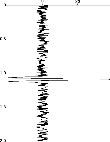

Estimating the noise level at $\sigma =$0.1,0.5, and 0.8 as before gives the signals depicted in Figure 8, Figure 9, and Figure 10 respectively. The first of these fit errors is impossible to achieve by means of the conjugate gradient algorithm at least with any reasonable number of iterations. The solution simply grows without bound, as one would expect, and retains almost no character of the target model (Figure 8). The correct estimate $\sigma = 0.5$ on the other hand gives you a reasonable estimate of the signal (Figure 9), with a bandlimited version of the spike dominating the series.

 

fig8 Figure 8 Signal estimate: target noise level 10%, unfiltered noise.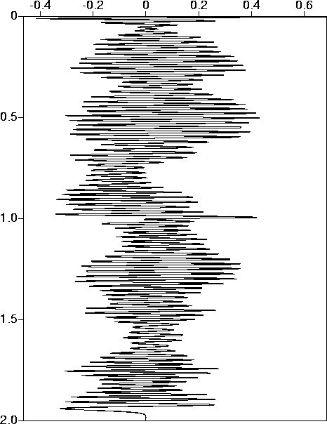

 

fig9 Figure 9 Signal estimate: target noise level 50%, unfiltered noise.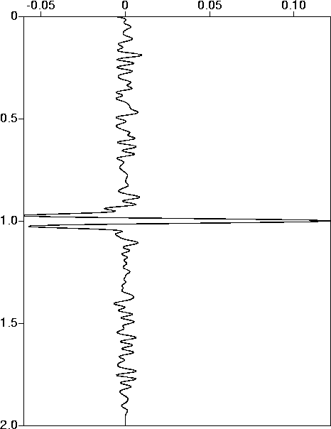

 

fig10 Figure 10 Signal estimate: target noise level 80%, unfiltered noise.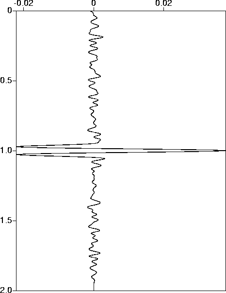

Again, the precise values of $\epsilon$ are inscrutable:

• $\sigma =$ 0.1 $\Rightarrow \epsilon =$ 8.87808e-11
• $\sigma =$ 0.5 $\Rightarrow \epsilon =$ 144.445
• $\sigma =$ 0.8 $\Rightarrow \epsilon =$ 405.233

The trend is even more marked here. The large out-of-band components in the data are essentially impossible to fit. So when you ask for a rather precise fit - 10% error - the weight on the model space decreases throughout the iteration, apparently with no end in sight. The value in the table above was the result of 10 Moré-Hebden iterations, and $\epsilon$ diminished by an order of magnitude or so each iteration. As soon as the level of fit permits you to discard the out of band components (that's what happened at $\sigma = 0.5$), the desired fit actually occurs and a reasonable value of $\epsilon$ results.

Clearly, prior knowledge of a reasonable model size would enable you to guess $\sigma$ in this example. However then you have to know the size of the model! This may be no more obvious than the size of the noise. This observation reinforces my contention that solution of problems like these demands that you know something in addition to the data samples - there is no ``born yesterday'' bootstrapping into a signal - noise distinction.