Synthetic data tests

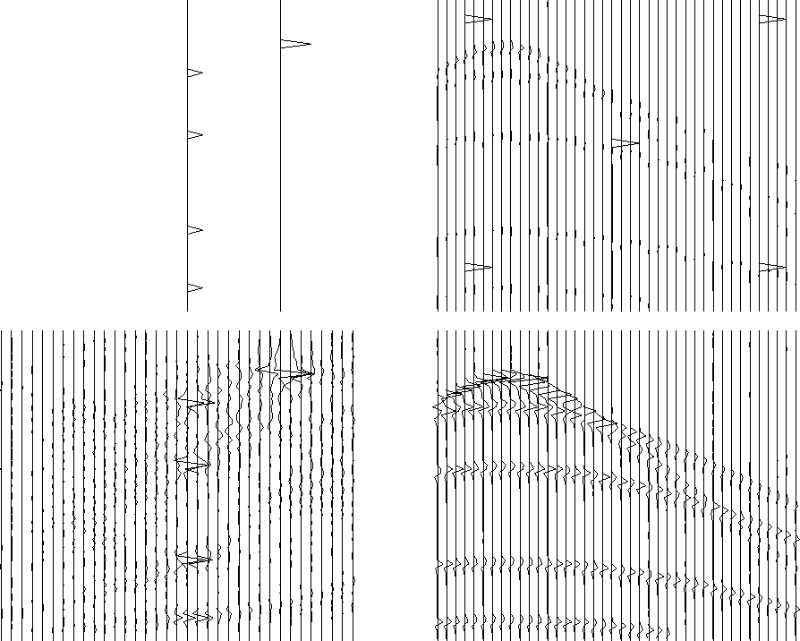
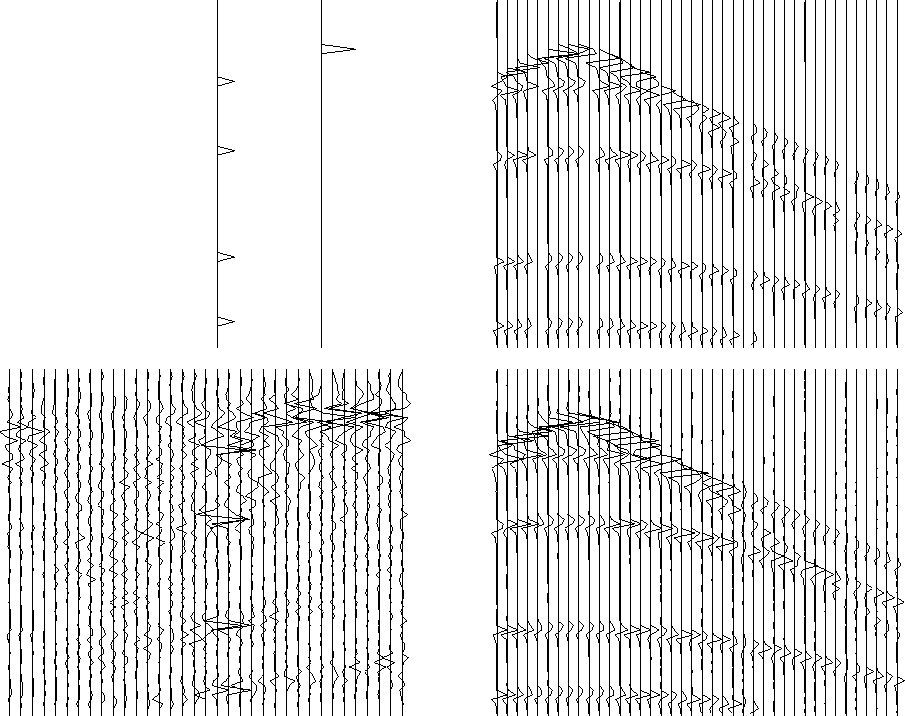
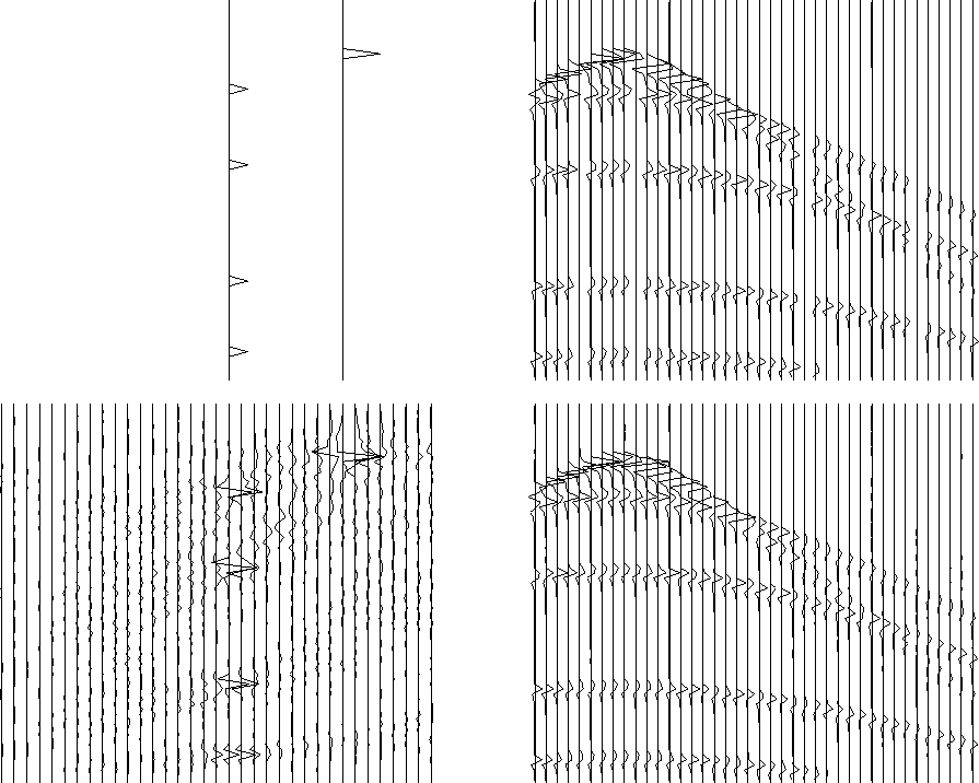
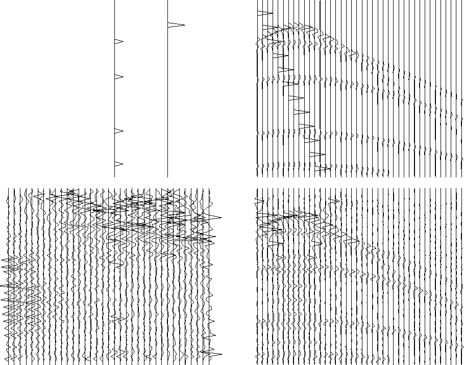
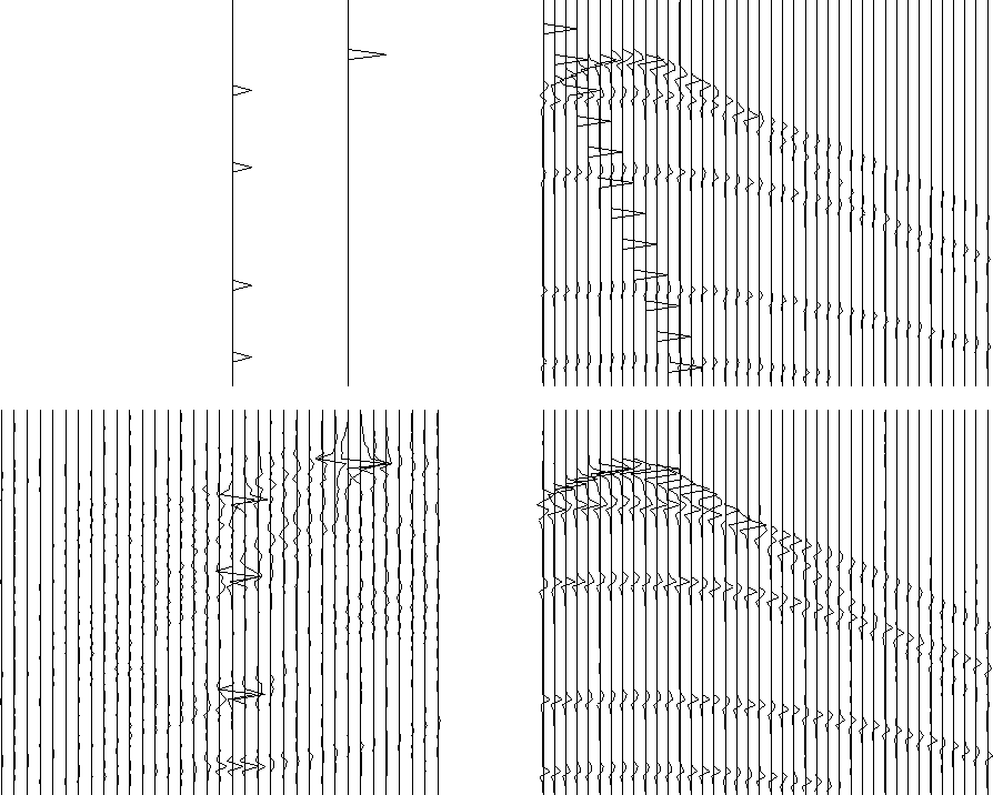
To compare the Huber function with the least squares measure, we generate a synthetic CMP gather (Figure 2) that we perturb by introducing: (1) missing traces, (2) a low velocity aliased plane wave, and (3) some sparsely distributed spiky noisy events. These data sets constitute the input for the iterative schemes ($\epsilon=0.01$ for each result). The panels display the model space on the left (after 20 iterations), and the data space on the right. The bottom right panels show the modeling of the last velocity result. All these results (Figures 4, 6, 8) prove the following: outcome of the Huber solver is insensitive to spiky events, like a pure l¹ norm misfit function. The outcome of the missing data problem was probably less predictable, but again, Huber copes more easily with the inconsistency introduced in the data.

 

datamodel Figure 2 Left: ideal velocity panel. Right: data model.

 

vel-miss2g
Figure 3 CG result with missing data.

 

vel-miss3h
Figure 4 Huber result with missing data.

 

vel-surf1g
Figure 5 CG result with a slow plane wave.

 

vel-surf2h
Figure 6 Huber result with a slow plane wave.

 

vel-spiky1g
Figure 7 CG result with spiky events.

 

vel-spiky2h
Figure 8 Huber result with spiky events.