SEARCHING THE SEA OF GALILEE

Figure 10 shows a bottom-sounding survey of the Sea of Galilee at various stages of processing. The ultimate goal is not only a good map of the depth to bottom, but images useful for the purpose of identifying archaeological, geological, or geophysical details of the sea bottom. The Sea of Galilee is unique because it is a fresh-water lake below sea-level. It seems to be connected to the great rift (pull-apart) valley crossing east Africa. We might delineate the Jordan River delta. We might find springs on the water bottom. We might find archaeological objects.

 

locfil90
Figure 10 Views of the bottom of the Sea of Galilee.

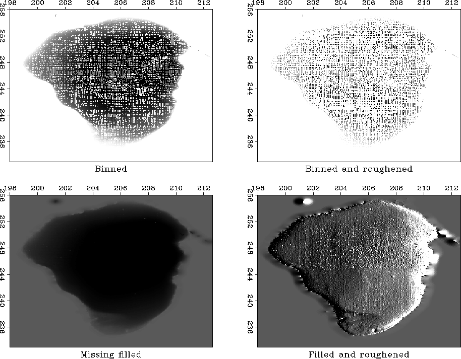The raw data is 132,044 triples, (x_i,y_i,z_i), where x_i ranges over about 12 km and where y_i ranges over about 20 km. The lines you see in Figure 10 are sequences of data points, i.e., the track of the survey vessel. The depths z_i are recorded to an accuracy of about 10 cm.

The first frame in Figure 10 shows simple binning. A coarser mesh would avoid the empty bins but lose resolution. As we refine the mesh for more detail, the number of empty bins grows as does the care needed in devising a technique for filling them. This first frame uses the simple idea from Chapter of spraying all the data values to the nearest bin with bin2() and dividing by the number in the bin. Bins with no data obviously need to be filled in some other way. I used a missing data program like that in the recent section on ``wells not matching the seismic map.'' Instead of roughening with a Laplacian, however, I used the gradient operator igrad2 The solver is grad2fill().  

module grad2fill {     # min r(m) = L J m + L known  where L is a lowcut filter.
  use igrad2
  use cgstep_mod
  use solver_mod
contains
  subroutine grad2fill2( niter, m1, m2, mm, mfixed) {
    integer,                    intent (in)     :: niter       # iterations
    integer,                    intent (in)     :: m1,m2       # data size
    logical, dimension (m1*m2), intent (in)     :: mfixed      # mask for known
    real,    dimension (m1*m2), intent (in out) :: mm          # model
    real,    dimension (m1*m2*2)                :: yy          # lowcut output
    call igrad2_init(m1,m2);                       yy = 0.     # initialize

call solver ( igrad2_lop, cgstep, mm, yy, niter,
                                      x0 = mm, known = mfixed )
    call cgstep_close ()
  }
}

The output of the roughening operator is an image, a filtered version of the depth, a filtered version of something real. Such filtering can enhance the appearance of interesting features. For example, scanning the shoreline of the roughened image (after missing data was filled), we see several ancient shorelines, now submerged.

The adjoint is the easiest image to build. The roughened map is a better image, often more informative than the map itself.

The views expose several defects of the data acquisition and of our data processing. The impulsive glitches (St. Peter's fish?) need to be removed but we must be careful not to throw out the sunken ships along with the bad data points. Even our best image shows clear evidence of the recording vessel's tracks. Strangely, some tracks are deeper than others. Perhaps the survey is assembled from work done in different seasons and the water level varied by season. Perhaps some days the vessel was more heavily loaded and the depth sounder was on a deeper keel.

A good image of the earth hides our data acquisition footprint.

We want the sharpest possible view of this classical site. A treasure hunt is never easy and no one guarantees we will find anything of great value but at least the exercise is a good warm-up for submarine petroleum exploration.