|
|
|
|
Fast log-decon with a quasi-Newton solver |
We define
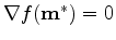
 a local minimizer for
 and we
assume that
and
satisfy the ``standard
requirements'':
and we
assume that
and
satisfy the ``standard
requirements'':
 is twice differentiable,
 ,
,
 is positive definite
, i.e.,
is positive definite
, i.e.,
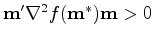 for all
 (
( denotes the adjoint).
 is the dimension of the model vector
  and
and
 the real space for the model vector
.
Any vector
the real space for the model vector
.
Any vector  that satisfies the standard requirements is a local
minimizer of
.
that satisfies the standard requirements is a local
minimizer of
.
Newton's method is an iterative process where the solution to the problem is updated as follows:
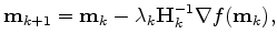 |
(1) |
 is the updated solution at iteration
 ,
,  the step length computed by a line search
that ensures a sufficient decrease of
and
the step length computed by a line search
that ensures a sufficient decrease of
and
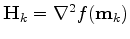 the Hessian (or second derivative). In many circumstances the inverse
of the Hessian can't be computed directly. It happens for example
when the matrix
the Hessian (or second derivative). In many circumstances the inverse
of the Hessian can't be computed directly. It happens for example
when the matrix  is too big or when operators are used
rather than matrices.
Fortunately we might be able to compute an approximation of
the Hessian of
. This strategy gives birth to quasi-Newton methods
where the way in which the Hessian is computed determines the method
(Kelley, 1999).
is too big or when operators are used
rather than matrices.
Fortunately we might be able to compute an approximation of
the Hessian of
. This strategy gives birth to quasi-Newton methods
where the way in which the Hessian is computed determines the method
(Kelley, 1999).
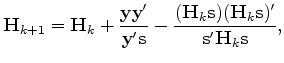
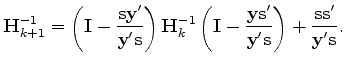
A possible update of the Hessian is given by the BFGS technique Fletcher (1970); Goldfarb (1970); Shanno (1970); Broyden (1969). The BFGS update is given by
 and
and
 .
In practice, however, we rather write the previous equation in terms of
the inverse matrices. We have then
.
In practice, however, we rather write the previous equation in terms of
the inverse matrices. We have then
 |
(3) |
 .
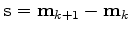
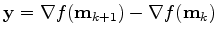
This requires that a gradient step vector
.
This requires that a gradient step vector  and a solution step
vector
and a solution step
vector  are kept in memory after each iteration.
Consequently this method might not been affordable with large data and
model space. In the next section
a modified version of the BFGS method that limits the storage needed
to compute the update of the Hessian is proposed.
are kept in memory after each iteration.
Consequently this method might not been affordable with large data and
model space. In the next section
a modified version of the BFGS method that limits the storage needed
to compute the update of the Hessian is proposed.
|
|
|
|
Fast log-decon with a quasi-Newton solver |